Saltar al contenido
GridBelt
  • Prueba de Excel
  • Práctica
  • Programas
  • Precios
Iniciar sesión
Empezar la prueba gratuita
  • Prueba de Excel
  • Práctica
  • Programas
  • Precios
Iniciar sesiónCrear cuenta
Empezar la prueba gratuita
GridBelt

Practica Excel en tu navegador.

Prueba de Excel

  • Nivel 1: Principiante
  • Nivel 2: Intermedio
  • Nivel 3: Experto
  • Prueba de Excel en 7 días
  • Clasificación
  • Prueba de Excel para entrevistas
  • Evaluación de Excel de Indeed

Práctica

  • Todos los ejercicios
  • Programas
  • Para principiantes

Guías

  • Fórmulas de Excel
  • Atajos de Excel

Empresa

  • Acerca de
  • Precios
  • Cómo corregimos

© GridBelt. Todos los derechos reservados.

  • Política de privacidad
  • Términos de uso
  • Política de reembolso

Excel es una marca comercial de Microsoft Corporation. Indeed, TestGorilla, SHL y otras marcas son propiedad de sus respectivos titulares. GridBelt es un sitio de práctica independiente y no está afiliado a Microsoft, TestGorilla, SHL ni Indeed, ni respaldado ni patrocinado por ellos.

  1. Práctica
  2. /
  3. Pivot tables

Pivot table practice: Count of Amount instead of Sum, find and fix the cause

  • Intermedio
  • ~12 min
  • Pivot tables

Enunciado en inglés

An assistant in the finance team built a PivotTable from the 150 October expense claims on the Claims sheet to show how much each department claimed. What she got is pictured below: her PivotTable Fields pane and a report with a single number labelled Count of Amount. Before the PivotTable is rebuilt, you check the Amount column with formulas, then answer four questions about fixing the report.

Left, the Pivot sheet: A1 Department with a filter drop-down showing (All), A3 Count of Amount, A4 142. Right, the PivotTable Fields pane: fields Claim ID, Date, Employee, Department (checked), Category, Amount (checked); Filters: Department; Columns: empty; Rows: empty; Values: Count of Amount, outlined in green.
The PivotTable as the assistant left it: the report (left) and its Fields pane (right).

Qué tienes que hacer

  1. 1Look at column F first: real numbers sit at the right edge of their cells. F2 and a number of other amounts sit at the left, the way text does, and a few claims have no amount at all.
  2. 2Click G2 and type =IF(F2="",0,VALUE(F2)): an empty amount becomes 0, VALUE turns text such as 233.54 into the number 233.54, and real numbers pass through unchanged. Fill G2 down to G151: select G2:G151 and press Ctrl+D (Windows) / ⌘D (Mac) — safer here than a double-click on the fill handle, which can stop early at the empty amounts in column F (the first is F6).
  3. 3Click J2 and count the cells of F2:F151 that hold text: =SUMPRODUCT(--ISTEXT(F2:F151)). ISTEXT returns TRUE for every text cell, the two minus signs turn TRUE/FALSE into 1/0, and SUMPRODUCT adds them up.
  4. 4Click J3 and total the cleaned column: =SUM(G2:G151). That is the number a Sum of Amount should report once column F holds real numbers.
  5. 5Then answer the four questions about the PivotTable and click Check.

Celdas de respuesta

Preguntas

Elige aquí tus respuestas: el botón Comprobar las corrige junto con las celdas de respuesta.

  1. Pregunta 1Which of these make Excel summarize Amount as Count instead of Sum when the field is dropped into Values? Select all that apply.

    Selecciona todas las que correspondan.

  2. Pregunta 2Suppose you change nothing in the data and only pick Sum in Value Field Settings, as pictured. What will Sum of Amount show?

    Elige una respuesta.

    Value Field Settings dialog for the Amount field: Source Name Amount, Custom Name Sum of Amount, tab Summarize Values By, list Sum (selected), Count, Average, Max, Min, Product; buttons Number Format, OK and Cancel.
  3. Pregunta 3A week later, 12 new claims are pasted below the list, in rows 152 to 163 (pictured). After Refresh the report still leaves them out. Which of these make the report include them? Select all that apply.

    Selecciona todas las que correspondan.

    The Claims sheet scrolled down under its frozen header row (Claim ID, Date, Employee, Department, Category, Amount). Rows 150 to 151 hold the last October claims, EXP-1149 to EXP-1150; rows 152 to 163 hold new claims EXP-1151 to EXP-1162, dated 2026-11-02 to 2026-11-06. A dashed outline marks A1:F151. Below, the Change PivotTable Data Source dialog: Select a table or range is chosen and the Table/Range box reads Claims!$A$1:$F$151.
    The Claims sheet after the paste, and the PivotTable's data source.
  4. Pregunta 4To list one row per department with its total, where should Department go in the Fields pane?

    Elige una respuesta.

Corrección

Responde a las preguntas, escribe tu fórmula en la cuadrícula, presiona Enter y luego haz clic en Comprobar. Evaluamos tus respuestas, el valor de cada celda de respuesta y la fórmula que lo produce.

Tareas

  1. Sin comprobarIn G2, turn the amount in F2 into a real number (0 when F2 is empty), then fill the formula down to G151.
  2. Sin comprobarIn J2, count how many cells in F2:F151 hold text instead of a number.
  3. Sin comprobarIn J3, add up the cleaned amounts in G2:G151.
  4. Sin comprobarPregunta 1: Which of these make Excel summarize Amount as Count instead of Sum when the field is dropped into Values? Select all that apply.
  5. Sin comprobarPregunta 2: Suppose you change nothing in the data and only pick Sum in Value Field Settings, as pictured. What will Sum of Amount show?
  6. Sin comprobarPregunta 3: A week later, 12 new claims are pasted below the list, in rows 152 to 163 (pictured). After Refresh the report still leaves them out. Which of these make the report include them? Select all that apply.
  7. Sin comprobarPregunta 4: To list one row per department with its total, where should Department go in the Fields pane?

Para las tareas de hoja de cálculo se recomienda una pantalla grande. La hoja se desplaza dentro de este recuadro.

StartInsertFormulasDataView
A1fxPreparando tu libro…
A
B
C
D
E
F
G
H
I
J
1
2
3
4
5
6
7
8
9
10
11
12
13
14
15
16
17
18
19
20
21
22
Sheet1

Responde a las preguntas, rellena las celdas y comprueba.

Sobre este ejercicio

Un conjunto de datos de 150 filas en una hoja, 3 celdas de respuesta, unos 12 minutos. Se corrige en tu navegador: el valor y la fórmula que lo produce, con comentarios que te dicen qué arreglar. Incluye además 4 preguntas de opción múltiple, que se corrigen con el mismo botón Comprobar.

Cómo resolverlo

  • G2=IF(F2="",0,VALUE(F2))
  • J2=SUMPRODUCT(--ISTEXT(F2:F151))
  • J3=SUM(G2:G151)

Excel sums a value field only when every cell of it is a number. Here some amounts are text (they sit at the left of the cell) and some are blank, so the PivotTable fell back to Count of Amount, which counts every non-empty cell like COUNTA. Picking Sum without cleaning adds the text amounts as 0, so the totals come out too low: convert them first (column G), then summarize by Sum. Department belongs in Rows for one row per department, and rows pasted below a fixed source range stay outside it until you change the data source, or use an Excel Table, which grows with the data.

In desktop Excel you can fix column F in place instead of using a helper column: select F2:F151 and use the warning button next to the green triangles → Convert to Number, or Data → Text to Columns → Finish, or copy a cell that holds 1 and use Paste Special → Multiply. VALUE reads text with your own regional settings; if your Excel uses a comma as the decimal separator, =NUMBERVALUE(F2,".") reads these dot-decimal amounts correctly. Blanks: fill them with 0 (Home → Find & Select → Go To Special → Blanks, type 0, Ctrl+Enter) or keep them and pick Sum yourself. A formula that returns "" for an empty amount returns text, which keeps the field on Count. Then refresh (PivotTable Analyze → Refresh, Alt+F5 on Windows; the tab is called Analyze in Excel 2016 and 2019) and set the field to Sum: right-click a value → Summarize Values By → Sum, or Value Field Settings. Change Data Source sits on the same tab; an Excel Table (Insert → Table) grows with every row added below it, so the PivotTable picks new rows up at the next Refresh. Auto Refresh, which Microsoft lists as a Microsoft 365 Insider feature for now, refreshes PivotTables on workbook data by itself, but it never stretches a fixed range either. This in-browser grid has no PivotTable: the pictures show what Excel does, and your formulas are graded in the grid.

Otras formas válidas

  • =F2*1 or =--F2 in G2 — arithmetic turns text into a number and an empty cell into 0
  • =COUNTIF(F2:F151,"*") or =COUNTA(F2:F151)-COUNT(F2:F151) in J2 — other ways to count the text cells
  • =SUMPRODUCT(--F2:F151) in J3 — the clean total in one formula, without column G

Respuestas a las preguntas
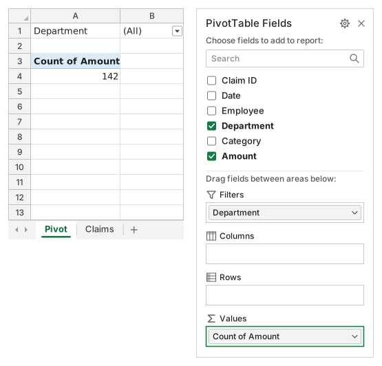
Left, the Pivot sheet: A1 Department with a filter drop-down showing (All), A3 Count of Amount, A4 142. Right, the PivotTable Fields pane: fields Claim ID, Date, Employee, Department (checked), Category, Amount (checked); Filters: Department; Columns: empty; Rows: empty; Values: Count of Amount, outlined in green.
The PivotTable as the assistant left it: the report (left) and its Fields pane (right).
  1. Pregunta 1. Which of these make Excel summarize Amount as Count instead of Sum when the field is dropped into Values? Select all that apply.

    Respuestas: Some amounts are stored as text y Some amount cells are blank

    Excel sums a value field only when every cell of it holds a number; text that looks like a number or an empty cell makes it fall back to Count, which counts non-empty cells like COUNTA (142 of the 150 claims here). Where Department sits, decimals and refreshing play no part in that choice.

  2. Pregunta 2. Suppose you change nothing in the data and only pick Sum in Value Field Settings, as pictured. What will Sum of Amount show?

    Respuesta: Too little: the text amounts are added as 0

    A PivotTable adds only real numbers: blank or nonnumeric values become 0 when the field is summed. The text amounts drop out of every total without any warning, so convert them first (your column G) and then summarize by Sum.

  3. Pregunta 3. A week later, 12 new claims are pasted below the list, in rows 152 to 163 (pictured). After Refresh the report still leaves them out. Which of these make the report include them? Select all that apply.

    Respuestas: Change Data Source so the range ends at row 163 y Make the claims an Excel Table and use it as the source

    The PivotTable reads the fixed range Claims!$A$1:$F$151, and Refresh or Refresh All re-reads exactly that range. Change Data Source extends it once; an Excel Table (Insert → Table, Ctrl+T on Windows, ⌘T on a Mac) grows with every row added below it, so each later Refresh picks new claims up.

  4. Pregunta 4. To list one row per department with its total, where should Department go in the Fields pane?

    Respuesta: Drag it to the Rows area

    A field in Rows gives each of its items its own line, here one per department with the amounts summed beside it and a Grand Total at the bottom. Columns would spread the departments across the top, Values would count them, and a report filter shows one total at a time.

Errores frecuentes

Picking Sum in Value Field Settings without cleaning the data: the text amounts are then added as 0 and every department total is too low. Converting with =IF(F2="","",VALUE(F2)) is the other trap: its "" results are text and keep the field on Count.

Cómo corregimos

Se acepta cualquier fórmula que produzca el resultado correcto, salvo que la tarea nombre una función: entonces otra función obtiene media puntuación. Comparamos los valores con una pequeña tolerancia y, en el texto, ignoramos mayúsculas y espacios. Un número correcto escrito a mano en lugar de una fórmula obtiene media puntuación. Las tareas de varias celdas obtienen la puntuación completa con el 100% de las celdas correctas y media puntuación desde el 50%. Cuando importa, también cambiamos una celda de entrada en una copia de tu hoja y comprobamos que tu fórmula se adapta.

Respuestas calculadas con las reglas de Excel 365 y comprobadas en nuestro corrector el 20 de noviembre de 2026. Autor: GridBelt team.

En estos programas

  • Excel test in 7 days, Plan del nivel 2Día 5
  • Excel test in 7 days, Plan del nivel 3Día 5
  • Excel for Data AnalystsDía 6

Ejercicios relacionados

  • Read a PivotTable report and check one of its cellsPrincipiante, ~8 min
  • Share of revenue by channel: % of Grand Total with formulasIntermedio, ~7 min
  • Count orders, names and blanks (COUNT, COUNTA, COUNTBLANK)Principiante, ~4 min

Referencia de la función

Documentación oficial

Siguiente ejercicio

Pick the right chart for each question