Vai al contenuto
GridBelt
  • Test Excel
  • Esercizi
  • Programmi
  • Prezzi
Accedi
Inizia il test gratuito
  • Test Excel
  • Esercizi
  • Programmi
  • Prezzi
AccediCrea un account
Inizia il test gratuito
GridBelt

Esercitati con Excel nel tuo browser.

Test Excel

  • Livello 1: Principiante
  • Livello 2: Intermedio
  • Livello 3: Esperto
  • Test Excel in 7 giorni
  • Classifica
  • Test Excel per il colloquio
  • Valutazione Excel di Indeed

Esercizi

  • Tutti gli esercizi
  • Programmi
  • Per principianti

Guide

  • Formule Excel
  • Scorciatoie Excel

Azienda

  • Chi siamo
  • Prezzi
  • Come valutiamo

© GridBelt. Tutti i diritti riservati.

  • Informativa sulla privacy
  • Termini di utilizzo
  • Politica di rimborso

Excel è un marchio di Microsoft Corporation. Indeed, TestGorilla, SHL e gli altri marchi appartengono ai rispettivi proprietari. GridBelt è un sito di esercitazione indipendente e non è affiliato a Microsoft, TestGorilla, SHL o Indeed, né approvato o sponsorizzato da queste società.

  1. Esercizi
  2. /
  3. Pivot tables

Pivot table practice: read a PivotTable report and check it with SUMIFS

  • Principiante
  • ~8 min
  • Pivot tables

Testo dell’esercizio in inglese

An office-supplies wholesaler closed 2025 with 210 orders, listed on the Orders sheet with region, quarter, product and amount. The sales manager summarised them in the PivotTable pictured below (the report on its own sheet and its PivotTable Fields pane) and wants to read it correctly before the board meeting. She also wants one number the report does not show: the average order behind one of its cells.

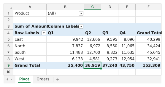
Immagine 1
PivotTable report on the Pivot sheet. Report filter in A1:B1: Product, (All). Row 3: Sum of Amount, Column Labels. Row 4: Row Labels, Q1, Q2, Q3, Q4, Grand Total. East: 9,942, 12,666, 9,595, 8,096; Grand Total 40,299. North: 7,837, 6,972, 8,550, 11,065; Grand Total 34,424. South: 11,488, 12,700, 9,822, 11,635; Grand Total 45,645. West: 6,133, 4,581, 9,273, 12,954; Grand Total 32,941. Grand Total row: 35,400, 36,919, 37,240, 43,750; overall 153,309. Cell C9 is selected.
The PivotTable on the Pivot sheet, built from the 210 orders on the Orders sheet.
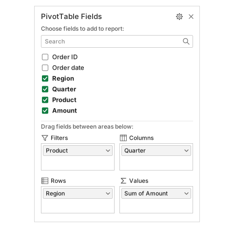
Immagine 2
PivotTable Fields pane. Fields: Order ID, Order date, Region (checked), Quarter (checked), Product (checked), Amount (checked). Filters: Product. Columns: Quarter. Rows: Region. Values: Sum of Amount.
The PivotTable Fields pane of the same report.

Cosa devi fare

  1. 1The report adds up the Amount of every order that falls under its row label and its column label. I2 and I3 name one of its cells — East and Q3 — and you rebuild that number from the 210 order lines in F2:F211.
  2. 2Click I4 and type =SUMIFS(F2:F211,C2:C211,I2,D2:D211,I3). SUMIFS takes the range to add first, then pairs of criteria range and criterion: Region (column C) must equal I2 and Quarter (column D) must equal I3. Press Enter and compare I4 with the East / Q3 number in the report.
  3. 3Click I5 and work out the average order of the same group, which the report does not show: =AVERAGEIFS(F2:F211,C2:C211,I2,D2:D211,I3), or divide I4 by =COUNTIFS(C2:C211,I2,D2:D211,I3).
  4. 4Point at I2 and I3 instead of typing "East" and "Q3" into the formulas: the checker switches them to another region and quarter and expects both answers to follow. Then answer the four questions about the report and click Check.

Celle di risposta

Domande

Scegli qui le tue risposte: il pulsante Verifica le valuta insieme alle celle di risposta.

  1. Domanda 1Look at the Fields pane: which part of the report does the field in its Columns area produce?

    Scegli una risposta.

  2. Domanda 2What does the number in C9 of the Pivot sheet, where the Grand Total row meets the Q2 column, show?

    Scegli una risposta.

  3. Domanda 3Which region brought in the largest amount over the whole year?

    Scegli una risposta.

  4. Domanda 4You want to see the individual orders behind the East / Q3 number. What is the quickest way in Excel?

    Scegli una risposta.

Correzione

Rispondi alle domande, scrivi la formula nella griglia, premi Enter, poi Verifica. Valutiamo le tue risposte, il valore in ogni cella di risposta e la formula che lo produce.

Attività

  1. Non verificatoIn I4, use SUMIFS to add up the Amount (F2:F211) of the orders whose Region equals I2 and whose Quarter equals I3 — the number the report shows for that cell.
  2. Non verificatoIn I5, calculate the average Amount of the same orders (Region = I2, Quarter = I3), a number the report does not show.
  3. Non verificatoDomanda 1: Look at the Fields pane: which part of the report does the field in its Columns area produce?
  4. Non verificatoDomanda 2: What does the number in C9 of the Pivot sheet, where the Grand Total row meets the Q2 column, show?
  5. Non verificatoDomanda 3: Which region brought in the largest amount over the whole year?
  6. Non verificatoDomanda 4: You want to see the individual orders behind the East / Q3 number. What is the quickest way in Excel?

Consigliato il computer per le attività sul foglio di calcolo. Il foglio scorre all’interno di questo riquadro.

StartInsertFormulasDataView
A1fxPreparazione della cartella di lavoro…
A
B
C
D
E
F
G
H
I
J
1
2
3
4
5
6
7
8
9
10
11
12
13
14
15
16
17
18
19
20
21
22
Sheet1

Rispondi alle domande, compila le celle, poi verifica.

Informazioni sull’esercizio

Un set di dati di 210 righe su un foglio, 2 celle di risposta, circa 8 minuti. Correzione nel tuo browser: il valore e la formula che lo produce, con indicazioni su cosa sistemare. L’esercizio include anche 4 domande a risposta multipla, valutate con lo stesso pulsante Verifica.

Come risolverlo

  • I4=SUMIFS(F2:F211,C2:C211,I2,D2:D211,I3)
  • I5=AVERAGEIFS(F2:F211,C2:C211,I2,D2:D211,I3)

A PivotTable value cell is a SUMIFS in disguise: it adds the Amount of the orders whose Region matches its row and whose Quarter matches its column, so =SUMIFS(F2:F211,C2:C211,I2,D2:D211,I3) reproduces the East / Q3 cell exactly, and AVERAGEIFS gives the average the report leaves out. Reading the report: the field in Columns (Quarter) makes the headings across the top and the field in Rows (Region) the labels down the side; the Grand Total row adds each column down (C9 is Q2 for all regions), the Grand Total column adds each row across, and F9 is the year. South leads the year although West has the biggest single quarter, and double-clicking any value cell lists the orders behind it.

Where it lives in Excel: Insert → PivotTable builds the report; the PivotTable Fields pane opens whenever a report cell is selected (PivotTable Analyze → Field List brings it back; the tab is called Analyze in Excel 2016 and 2019). Show Details: double-click a value or right-click → Show Details, and the rows behind it land on a new sheet (PivotTable Options → Data → Enable show details switches this off). To show averages in the report itself, add Amount to Values a second time and set Value Field Settings → Summarize value field by → Average. Pitfall 1: the report is a snapshot of the source; after the orders change, click Refresh (PivotTable Analyze → Refresh, Alt+F5 on Windows). Auto Refresh, which Microsoft lists as a Microsoft 365 Insider feature for now, updates PivotTables on workbook data by itself; without it the report waits for Refresh. Pitfall 2: clicking a report cell while you type a formula inserts a GETPIVOTDATA formula such as =GETPIVOTDATA("Amount",Pivot!$A$3,"Region","East","Quarter","Q3") instead of a plain reference; it keeps pointing at the right number when the report changes shape, and PivotTable Analyze → Options → Generate GetPivotData turns it off. Pitfall 3: the biggest number in the grid is a single cell, not the best region; compare the Grand Total column. This in-browser grid has no PivotTable: the report is a picture drawn from the same 210 orders, and your SUMIFS and AVERAGEIFS formulas are graded in the grid.

Altri metodi validi

  • =SUMPRODUCT((C2:C211=I2)*(D2:D211=I3)*F2:F211) — the array form of the same sum
  • =I4/COUNTIFS(C2:C211,I2,D2:D211,I3) — the average as the sum divided by the number of orders
  • =AVERAGE(FILTER(F2:F211,(C2:C211=I2)*(D2:D211=I3))) — Excel 365 only

Risposte alle domande
PivotTable report on the Pivot sheet. Report filter in A1:B1: Product, (All). Row 3: Sum of Amount, Column Labels. Row 4: Row Labels, Q1, Q2, Q3, Q4, Grand Total. East: 9,942, 12,666, 9,595, 8,096; Grand Total 40,299. North: 7,837, 6,972, 8,550, 11,065; Grand Total 34,424. South: 11,488, 12,700, 9,822, 11,635; Grand Total 45,645. West: 6,133, 4,581, 9,273, 12,954; Grand Total 32,941. Grand Total row: 35,400, 36,919, 37,240, 43,750; overall 153,309. Cell C9 is selected.
The PivotTable on the Pivot sheet, built from the 210 orders on the Orders sheet.
PivotTable Fields pane. Fields: Order ID, Order date, Region (checked), Quarter (checked), Product (checked), Amount (checked). Filters: Product. Columns: Quarter. Rows: Region. Values: Sum of Amount.
The PivotTable Fields pane of the same report.
  1. Domanda 1. Look at the Fields pane: which part of the report does the field in its Columns area produce?

    Risposta: The Q1 to Q4 headings across the top

    Quarter sits in the Columns area, and a field in Columns turns its items into the headings across the top of the report. Region in Rows gives the labels down the side, Amount in Values the numbers, and Product in Filters the (All) box above.

  2. Domanda 2. What does the number in C9 of the Pivot sheet, where the Grand Total row meets the Q2 column, show?

    Risposta: The Q2 amount of all four regions added together

    The Grand Total row adds each column down: C9 = 12,666 + 6,972 + 12,700 + 4,581 = 36,919. The whole year of every region is the bottom-right cell F9, and a number of orders would need Count instead of Sum.

  3. Domanda 3. Which region brought in the largest amount over the whole year?

    Risposta: South

    Read the Grand Total column (F5:F8): South has the largest year, 45,645. West owns the biggest single number in the report (12,954 in Q4) but its year adds up to only 32,941.

  4. Domanda 4. You want to see the individual orders behind the East / Q3 number. What is the quickest way in Excel?

    Risposta: Double-click that value cell

    Double-clicking a value cell (or right-click → Show Details) puts the orders behind that number on a new worksheet. Refresh only re-reads the source data, Order ID in Values would count the orders, and PivotTable cells hold no formula to open.

Errori comuni

Typing the criteria into the formula, =SUMIFS(F2:F211,C2:C211,"East",D2:D211,"Q3"): the value matches today, but the checker switches I2 and I3 and the hard-coded formula does not follow.

Come valutiamo

È accettata qualsiasi formula che produce il risultato giusto, a meno che l’attività non indichi una funzione: in quel caso un’altra funzione vale metà dei punti. Confrontiamo i valori con una piccola tolleranza e ignoriamo maiuscole, minuscole e spazi nel testo. Un numero corretto digitato a mano invece di una formula vale metà dei punti. Le attività su più celle valgono il punteggio pieno con il 100% delle celle giuste, metà dei punti dal 50%. Dove serve, cambiamo anche una cella di input su una copia del tuo foglio e controlliamo che la formula si aggiorni.

Risposte calcolate con le regole di Excel 365 e verificate nel nostro correttore in data 20 novembre 2026. Autore: GridBelt team.

In questi programmi

  • Excel for Administrative AssistantsGiorno 7
  • Learn Excel From ScratchGiorno 8

Esercizi correlati

  • Pivot without a pivot: revenue by category and month with SUMIFSIntermedio, ~10 min
  • Sales by region and product with SUMIFSIntermedio, ~7 min
  • Fix a PivotTable that counts instead of sumsIntermedio, ~12 min

Guida alla funzione

Documentazione ufficiale

Esercizio successivo

Fix a PivotTable that counts instead of sums