Pular para o conteúdo
GridBelt
  • Teste de Excel
  • Prática
  • Programas
  • Preços
Entrar
Começar o teste gratuito
  • Teste de Excel
  • Prática
  • Programas
  • Preços
EntrarCriar conta
Começar o teste gratuito
GridBelt

Pratique Excel no seu navegador.

Teste de Excel

  • Nível 1: Iniciante
  • Nível 2: Intermediário
  • Nível 3: Avançado
  • Teste de Excel em 7 dias
  • Ranking
  • Teste de Excel para entrevista
  • Avaliação de Excel da Indeed

Prática

  • Todos os exercícios
  • Programas
  • Para iniciantes

Guias

  • Fórmulas do Excel
  • Atalhos do Excel

Empresa

  • Sobre nós
  • Preços
  • Como corrigimos

© GridBelt. Todos os direitos reservados.

  • Política de Privacidade
  • Termos de Uso
  • Política de Reembolso

Excel é uma marca comercial da Microsoft Corporation. Indeed, TestGorilla, SHL e outras marcas pertencem aos seus respectivos proprietários. O GridBelt é um site de prática independente e não tem afiliação com Microsoft, TestGorilla, SHL ou Indeed, nem é endossado ou patrocinado por eles.

  1. Prática
  2. /
  3. Pivot tables

Pivot table practice: read a PivotTable report and check it with SUMIFS

  • Iniciante
  • ~8 min
  • Pivot tables

Enunciado em inglês

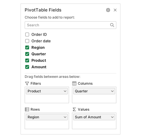
An office-supplies wholesaler closed 2025 with 210 orders, listed on the Orders sheet with region, quarter, product and amount. The sales manager summarised them in the PivotTable pictured below (the report on its own sheet and its PivotTable Fields pane) and wants to read it correctly before the board meeting. She also wants one number the report does not show: the average order behind one of its cells.

Imagem 1
PivotTable report on the Pivot sheet. Report filter in A1:B1: Product, (All). Row 3: Sum of Amount, Column Labels. Row 4: Row Labels, Q1, Q2, Q3, Q4, Grand Total. East: 9,942, 12,666, 9,595, 8,096; Grand Total 40,299. North: 7,837, 6,972, 8,550, 11,065; Grand Total 34,424. South: 11,488, 12,700, 9,822, 11,635; Grand Total 45,645. West: 6,133, 4,581, 9,273, 12,954; Grand Total 32,941. Grand Total row: 35,400, 36,919, 37,240, 43,750; overall 153,309. Cell C9 is selected.
The PivotTable on the Pivot sheet, built from the 210 orders on the Orders sheet.
Imagem 2
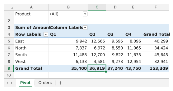
PivotTable Fields pane. Fields: Order ID, Order date, Region (checked), Quarter (checked), Product (checked), Amount (checked). Filters: Product. Columns: Quarter. Rows: Region. Values: Sum of Amount.
The PivotTable Fields pane of the same report.

O que você precisa fazer

  1. 1The report adds up the Amount of every order that falls under its row label and its column label. I2 and I3 name one of its cells — East and Q3 — and you rebuild that number from the 210 order lines in F2:F211.
  2. 2Click I4 and type =SUMIFS(F2:F211,C2:C211,I2,D2:D211,I3). SUMIFS takes the range to add first, then pairs of criteria range and criterion: Region (column C) must equal I2 and Quarter (column D) must equal I3. Press Enter and compare I4 with the East / Q3 number in the report.
  3. 3Click I5 and work out the average order of the same group, which the report does not show: =AVERAGEIFS(F2:F211,C2:C211,I2,D2:D211,I3), or divide I4 by =COUNTIFS(C2:C211,I2,D2:D211,I3).
  4. 4Point at I2 and I3 instead of typing "East" and "Q3" into the formulas: the checker switches them to another region and quarter and expects both answers to follow. Then answer the four questions about the report and click Check.

Células de resposta

Questões

Escolha suas respostas aqui: o botão Verificar as corrige junto com as células de resposta.

  1. Questão 1Look at the Fields pane: which part of the report does the field in its Columns area produce?

    Escolha uma resposta.

  2. Questão 2What does the number in C9 of the Pivot sheet, where the Grand Total row meets the Q2 column, show?

    Escolha uma resposta.

  3. Questão 3Which region brought in the largest amount over the whole year?

    Escolha uma resposta.

  4. Questão 4You want to see the individual orders behind the East / Q3 number. What is the quickest way in Excel?

    Escolha uma resposta.

Correção

Responda às questões, digite sua fórmula na grade, pressione Enter e depois clique em Verificar. Avaliamos suas respostas, o valor de cada célula de resposta e a fórmula por trás dele.

Tarefas

  1. Não verificadoIn I4, use SUMIFS to add up the Amount (F2:F211) of the orders whose Region equals I2 and whose Quarter equals I3 — the number the report shows for that cell.
  2. Não verificadoIn I5, calculate the average Amount of the same orders (Region = I2, Quarter = I3), a number the report does not show.
  3. Não verificadoQuestão 1: Look at the Fields pane: which part of the report does the field in its Columns area produce?
  4. Não verificadoQuestão 2: What does the number in C9 of the Pivot sheet, where the Grand Total row meets the Q2 column, show?
  5. Não verificadoQuestão 3: Which region brought in the largest amount over the whole year?
  6. Não verificadoQuestão 4: You want to see the individual orders behind the East / Q3 number. What is the quickest way in Excel?

Recomendamos um computador para as tarefas de planilha. A planilha rola dentro desta caixa.

StartInsertFormulasDataView
A1fxPreparando sua pasta de trabalho…
A
B
C
D
E
F
G
H
I
J
1
2
3
4
5
6
7
8
9
10
11
12
13
14
15
16
17
18
19
20
21
22
Sheet1

Responda às questões, preencha as células e verifique.

Sobre este exercício

Um conjunto de dados de 210 linhas em uma planilha, 2 células de resposta, cerca de 8 minutos. Corrigido no seu navegador: o valor e a fórmula por trás dele, com feedback que mostra o que corrigir. O exercício também traz 4 questões de múltipla escolha, corrigidas pelo mesmo botão Verificar.

Como resolver

  • I4=SUMIFS(F2:F211,C2:C211,I2,D2:D211,I3)
  • I5=AVERAGEIFS(F2:F211,C2:C211,I2,D2:D211,I3)

A PivotTable value cell is a SUMIFS in disguise: it adds the Amount of the orders whose Region matches its row and whose Quarter matches its column, so =SUMIFS(F2:F211,C2:C211,I2,D2:D211,I3) reproduces the East / Q3 cell exactly, and AVERAGEIFS gives the average the report leaves out. Reading the report: the field in Columns (Quarter) makes the headings across the top and the field in Rows (Region) the labels down the side; the Grand Total row adds each column down (C9 is Q2 for all regions), the Grand Total column adds each row across, and F9 is the year. South leads the year although West has the biggest single quarter, and double-clicking any value cell lists the orders behind it.

Where it lives in Excel: Insert → PivotTable builds the report; the PivotTable Fields pane opens whenever a report cell is selected (PivotTable Analyze → Field List brings it back; the tab is called Analyze in Excel 2016 and 2019). Show Details: double-click a value or right-click → Show Details, and the rows behind it land on a new sheet (PivotTable Options → Data → Enable show details switches this off). To show averages in the report itself, add Amount to Values a second time and set Value Field Settings → Summarize value field by → Average. Pitfall 1: the report is a snapshot of the source; after the orders change, click Refresh (PivotTable Analyze → Refresh, Alt+F5 on Windows). Auto Refresh, which Microsoft lists as a Microsoft 365 Insider feature for now, updates PivotTables on workbook data by itself; without it the report waits for Refresh. Pitfall 2: clicking a report cell while you type a formula inserts a GETPIVOTDATA formula such as =GETPIVOTDATA("Amount",Pivot!$A$3,"Region","East","Quarter","Q3") instead of a plain reference; it keeps pointing at the right number when the report changes shape, and PivotTable Analyze → Options → Generate GetPivotData turns it off. Pitfall 3: the biggest number in the grid is a single cell, not the best region; compare the Grand Total column. This in-browser grid has no PivotTable: the report is a picture drawn from the same 210 orders, and your SUMIFS and AVERAGEIFS formulas are graded in the grid.

Outras formas que funcionam

  • =SUMPRODUCT((C2:C211=I2)*(D2:D211=I3)*F2:F211) — the array form of the same sum
  • =I4/COUNTIFS(C2:C211,I2,D2:D211,I3) — the average as the sum divided by the number of orders
  • =AVERAGE(FILTER(F2:F211,(C2:C211=I2)*(D2:D211=I3))) — Excel 365 only

Respostas às questões
PivotTable report on the Pivot sheet. Report filter in A1:B1: Product, (All). Row 3: Sum of Amount, Column Labels. Row 4: Row Labels, Q1, Q2, Q3, Q4, Grand Total. East: 9,942, 12,666, 9,595, 8,096; Grand Total 40,299. North: 7,837, 6,972, 8,550, 11,065; Grand Total 34,424. South: 11,488, 12,700, 9,822, 11,635; Grand Total 45,645. West: 6,133, 4,581, 9,273, 12,954; Grand Total 32,941. Grand Total row: 35,400, 36,919, 37,240, 43,750; overall 153,309. Cell C9 is selected.
The PivotTable on the Pivot sheet, built from the 210 orders on the Orders sheet.
PivotTable Fields pane. Fields: Order ID, Order date, Region (checked), Quarter (checked), Product (checked), Amount (checked). Filters: Product. Columns: Quarter. Rows: Region. Values: Sum of Amount.
The PivotTable Fields pane of the same report.
  1. Questão 1. Look at the Fields pane: which part of the report does the field in its Columns area produce?

    Resposta: The Q1 to Q4 headings across the top

    Quarter sits in the Columns area, and a field in Columns turns its items into the headings across the top of the report. Region in Rows gives the labels down the side, Amount in Values the numbers, and Product in Filters the (All) box above.

  2. Questão 2. What does the number in C9 of the Pivot sheet, where the Grand Total row meets the Q2 column, show?

    Resposta: The Q2 amount of all four regions added together

    The Grand Total row adds each column down: C9 = 12,666 + 6,972 + 12,700 + 4,581 = 36,919. The whole year of every region is the bottom-right cell F9, and a number of orders would need Count instead of Sum.

  3. Questão 3. Which region brought in the largest amount over the whole year?

    Resposta: South

    Read the Grand Total column (F5:F8): South has the largest year, 45,645. West owns the biggest single number in the report (12,954 in Q4) but its year adds up to only 32,941.

  4. Questão 4. You want to see the individual orders behind the East / Q3 number. What is the quickest way in Excel?

    Resposta: Double-click that value cell

    Double-clicking a value cell (or right-click → Show Details) puts the orders behind that number on a new worksheet. Refresh only re-reads the source data, Order ID in Values would count the orders, and PivotTable cells hold no formula to open.

Erros comuns

Typing the criteria into the formula, =SUMIFS(F2:F211,C2:C211,"East",D2:D211,"Q3"): the value matches today, but the checker switches I2 and I3 and the hard-coded formula does not follow.

Como corrigimos

Qualquer fórmula que produza o resultado certo é aceita, a menos que a tarefa cite uma função: nesse caso, outra função vale metade da pontuação. Comparamos os valores com uma pequena tolerância e ignoramos maiúsculas e espaços no texto. Um número certo digitado à mão em vez de uma fórmula vale metade da pontuação. Tarefas com várias células valem a pontuação integral com 100% das células certas e metade a partir de 50%. Quando faz diferença, também mudamos uma célula de entrada em uma cópia da sua planilha e verificamos se sua fórmula acompanha.

Respostas calculadas com as regras do Excel 365 e verificadas no nosso corretor em 20 de novembro de 2026. Autor: GridBelt team.

Nestes programas

  • Excel for Administrative AssistantsDia 7
  • Learn Excel From ScratchDia 8

Exercícios relacionados

  • Pivot without a pivot: revenue by category and month with SUMIFSIntermediário, ~10 min
  • Sales by region and product with SUMIFSIntermediário, ~7 min
  • Fix a PivotTable that counts instead of sumsIntermediário, ~12 min

Referência da função

Documentação oficial

Próximo exercício

Fix a PivotTable that counts instead of sums