Zum Inhalt springen
GridBelt
  • Excel-Test
  • Übungen
  • Programme
  • Preise
Anmelden
Kostenlosen Test starten
  • Excel-Test
  • Übungen
  • Programme
  • Preise
AnmeldenKonto erstellen
Kostenlosen Test starten
GridBelt

Excel üben – direkt im Browser.

Excel-Test

  • Stufe 1: Anfänger
  • Stufe 2: Fortgeschrittene
  • Stufe 3: Experten
  • Excel-Test in 7 Tagen
  • Bestenliste
  • Excel-Test im Bewerbungsverfahren
  • Excel-Test von Indeed

Übungen

  • Alle Übungen
  • Programme
  • Für Anfänger

Ratgeber

  • Excel-Formeln
  • Excel-Tastenkombinationen

Unternehmen

  • Über uns
  • Preise
  • So bewerten wir

© GridBelt. Alle Rechte vorbehalten.

  • Datenschutzerklärung
  • Nutzungsbedingungen
  • Rückerstattungsrichtlinie

Excel ist eine Marke der Microsoft Corporation. Indeed, TestGorilla, SHL und andere Marken sind Eigentum ihrer jeweiligen Inhaber. GridBelt ist eine unabhängige Übungsplattform, steht mit Microsoft, TestGorilla, SHL oder Indeed in keiner Verbindung und wird von keinem dieser Unternehmen unterstützt oder gesponsert.

  1. Übungen
  2. /
  3. Charts

Excel chart practice: read a clustered column chart of revenue by region

  • Anfänger
  • ~6 Min.
  • Charts

Übungstext auf Englisch

A kitchen-appliance wholesaler sells in six US regions. Before the sales kick-off, the director looks at a clustered column chart of revenue by region for 2025 and 2026, built from the table in A1:C8; the Total row adds up the regions. Read the chart to answer the questions, and put each growth rate next to the table: the chart shows dollars, not percentages.

Clustered column chart "Revenue by region ($ thousands)" with two columns per region, a blue one for 2025 and an orange one for 2026 (legend below the chart), each labelled with its value in thousands of dollars on an axis that starts at 0. Six regions from left to right, 2025 then 2026: Northeast 842 and 879; Southeast 612 and 689; Midwest 575 and 531; Southwest 403 and 446; Mountain 186 and 225; Pacific 736 and 771.

Ihre Aufgabe

  1. 1The table A1:C8 holds the numbers behind the chart: one row per region with its 2025 revenue in column B and its 2026 revenue in column C, and the Total row 8.
  2. 2Click D2. Growth is the change divided by the starting year: subtract the 2025 revenue (B2) from the 2026 revenue (C2), put brackets around the difference and divide by B2.
  3. 3Press Enter and fill D2 down to D8 (double-click the fill handle or press Ctrl+D / ⌘D on the selected range), so the Total row gets the company's growth too.
  4. 4Select D2:D8 and apply a percentage format with one decimal place: Ctrl+Shift+% (Control+Shift+% on a Mac), then Increase Decimal once (in this grid: the toolbar's Increase decimal places button, under ⋮ when the toolbar is narrow; in Excel, Format Cells with Ctrl+1 / ⌘1 → Percentage → 1 decimal place works too). A fall shows as a negative percentage.
  5. 5Then answer the questions: the first three need only the chart, the last one uses your column D. The chart is a picture: this practice grid has no chart command.

Antwortzellen

Fragen

Wählen Sie hier Ihre Antworten. „Prüfen“ bewertet sie zusammen mit den Antwortzellen.

  1. Frage 1In the chart, what do the orange columns show?

    Wählen Sie eine Antwort.

  2. Frage 2Judging by the chart, which region added the most revenue in dollars from 2025 to 2026?

    Wählen Sie eine Antwort.

  3. Frage 3Which region's revenue fell from 2025 to 2026?

    Wählen Sie eine Antwort.

  4. Frage 4Now look at your column D. Which regions grew faster in percent than the company as a whole (the Total row)? Select all that apply.

    Wählen Sie alle zutreffenden Antworten.

Feedback

Beantworten Sie die Fragen, geben Sie Ihre Formel in die Tabelle ein, drücken Sie Enter und dann „Prüfen“. Wir bewerten Ihre Antworten, den Wert in jeder Antwortzelle und die Formel dahinter.

Aufgaben

  1. Nicht geprüftIn D2:D8, compute each row's growth from 2025 to 2026, (2026 − 2025) ÷ 2025, with one formula filled down through the Total row.
  2. Nicht geprüftFormat D2:D8 as a percentage with one decimal place (for example 4.4% or -7.6%).
  3. Nicht geprüftFrage 1: In the chart, what do the orange columns show?
  4. Nicht geprüftFrage 2: Judging by the chart, which region added the most revenue in dollars from 2025 to 2026?
  5. Nicht geprüftFrage 3: Which region's revenue fell from 2025 to 2026?
  6. Nicht geprüftFrage 4: Now look at your column D. Which regions grew faster in percent than the company as a whole (the Total row)? Select all that apply.

Für Tabellenaufgaben empfehlen wir einen Computer. Die Tabelle scrollt innerhalb dieses Rahmens.

StartInsertFormulasDataView
A1fxIhre Arbeitsmappe wird vorbereitet…
A
B
C
D
E
F
G
H
I
J
1
2
3
4
5
6
7
8
9
10
11
12
13
14
15
16
17
18
19
20
21
22
Sheet1

Beantworten Sie die Fragen, füllen Sie die Zellen aus und prüfen Sie.

Über diese Übung

Ein Datensatz mit 7 Zeilen auf einem Tabellenblatt, eine Antwortzelle, etwa 6 Minuten. Bewertet in Ihrem Browser: der Wert und die Formel dahinter, mit Feedback, das die Korrektur benennt. Dazu kommen 4 Multiple-Choice-Fragen, die ebenfalls mit „Prüfen“ bewertet werden.

So lösen Sie die Aufgabe

  • D2=(C2-B2)/B2

Growth is the change divided by the starting value: =(C2-B2)/B2 gives the first region's 2026 change as a share of 2025, and filling down to the Total row gives the company's rate to compare with; the 0.0% format shows 0.044 as 4.4%. Reading the chart: the legend says orange is 2026; the biggest dollar increase is the widest gap between a region's two columns (Southeast); the only orange column shorter than its blue partner is Midwest's; and column D shows that Southeast, Southwest and Mountain grew faster than the company.

In Excel: select A1:C7 (leave the Total row out, or its two columns dwarf every region) and choose Insert → Insert Column or Bar Chart → Clustered Column; Excel makes the two year columns the series because the range has more rows than columns. Data labels: Chart Design → Add Chart Element → Data Labels (the tab is called Design, under Chart Tools, in Excel 2016–2019); the number format code #,##0, (Format Axis or Format Data Labels → Number) shows thousands, 879,400 as 879. Pitfall 1: a chart compares heights, so it shows dollar differences; growth in percent needs the calculation, and a small region can grow fastest with the shortest columns. Pitfall 2: if the year headers were numbers instead of text, Excel could plot them as data; clearing the corner cell A1 or storing the years as text keeps them as series names (fix an existing chart with Chart Design → Select Data). Pitfall 3: =C2-B2/B2 without brackets divides first and returns a huge number instead of a percentage.

Andere Wege, die funktionieren

  • =C2/B2-1 — the same result, shorter
  • =(C2-B2)/ABS(B2) — also right when a starting value can be negative (not the case for revenue)
  • =IFERROR((C2-B2)/B2,"") — blank instead of #DIV/0! for a region that is new this year

Antworten auf die Fragen
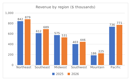
Clustered column chart "Revenue by region ($ thousands)" with two columns per region, a blue one for 2025 and an orange one for 2026 (legend below the chart), each labelled with its value in thousands of dollars on an axis that starts at 0. Six regions from left to right, 2025 then 2026: Northeast 842 and 879; Southeast 612 and 689; Midwest 575 and 531; Southwest 403 and 446; Mountain 186 and 225; Pacific 736 and 771.
  1. Frage 1. In the chart, what do the orange columns show?

    Antwort: Revenue in 2026

    The legend under the chart maps each colour to a series: blue is 2025 and orange is 2026. A clustered column chart draws one column per series in every category, side by side, so each region gets a 2025 column and a 2026 column.

  2. Frage 2. Judging by the chart, which region added the most revenue in dollars from 2025 to 2026?

    Antwort: Southeast region

    Compare the gap between each region's two columns, not the height of the orange one: Southeast goes from about 612 to 689 thousand, about $78K more, the widest gap. Northeast has the tallest columns but adds only about $37K.

  3. Frage 3. Which region's revenue fell from 2025 to 2026?

    Antwort: Midwest region

    Midwest is the only region whose orange 2026 column is shorter than its blue 2025 column (about 575 down to 531 thousand). Mountain has the shortest columns, but small is not the same as falling: its 2026 column is the taller of its pair.

  4. Frage 4. Now look at your column D. Which regions grew faster in percent than the company as a whole (the Total row)? Select all that apply.

    Antworten: Southeast region, Southwest region und Mountain region

    The company grew by 5.6%. Southeast (12.7%), Southwest (10.8%) and Mountain (20.6%) beat that. Mountain has the highest rate of all although its columns are the shortest: a percentage divides the increase by the starting value, and a small start makes a modest gain a big percentage.

Häufige Fehler

Typing =C2-B2/B2 without brackets: Excel divides B2 by itself first and returns the 2026 revenue minus 1 (879,399 for Northeast) instead of a growth rate. Wrap the difference in brackets: =(C2-B2)/B2.

So bewerten wir

Jede Formel, die das richtige Ergebnis liefert, wird akzeptiert, außer die Aufgabe nennt eine Funktion: Dann bringt eine andere Funktion die halbe Punktzahl. Wir vergleichen Werte mit einer kleinen Toleranz und ignorieren bei Text Groß- und Kleinschreibung sowie Leerzeichen. Eine richtige Zahl, die statt einer Formel von Hand eingetippt wurde, bringt die halbe Punktzahl. Aufgaben mit mehreren Zellen bringen die volle Punktzahl, wenn 100% der Zellen stimmen, und die halbe ab 50%. Wo es darauf ankommt, ändern wir außerdem eine Eingabezelle in einer Kopie Ihrer Tabelle und prüfen, ob Ihre Formel mitzieht.

Antworten nach den Regeln von Excel 365 berechnet und am 20. November 2026 in unserem Bewertungssystem geprüft. Verfasst von GridBelt team.

In diesen Programmen

  • Learn Excel From ScratchTag 2

Ähnliche Übungen

  • Year-over-year % changeAnfänger, ~4 Min.
  • Pick the right chart for each questionAnfänger, ~9 Min.
  • Spot a misleading chart axis and measure the real differenceFortgeschrittene, ~8 Min.

Funktionsreferenz

Offizielle Dokumentation

Nächste Übung

Spot a misleading chart axis and measure the real difference