Zum Inhalt springen
GridBelt
  • Excel-Test
  • Übungen
  • Programme
  • Preise
Anmelden
Kostenlosen Test starten
  • Excel-Test
  • Übungen
  • Programme
  • Preise
AnmeldenKonto erstellen
Kostenlosen Test starten
GridBelt

Excel üben – direkt im Browser.

Excel-Test

  • Stufe 1: Anfänger
  • Stufe 2: Fortgeschrittene
  • Stufe 3: Experten
  • Excel-Test in 7 Tagen
  • Bestenliste
  • Excel-Test im Bewerbungsverfahren
  • Excel-Test von Indeed

Übungen

  • Alle Übungen
  • Programme
  • Für Anfänger

Ratgeber

  • Excel-Formeln
  • Excel-Tastenkombinationen

Unternehmen

  • Über uns
  • Preise
  • So bewerten wir

© GridBelt. Alle Rechte vorbehalten.

  • Datenschutzerklärung
  • Nutzungsbedingungen
  • Rückerstattungsrichtlinie

Excel ist eine Marke der Microsoft Corporation. Indeed, TestGorilla, SHL und andere Marken sind Eigentum ihrer jeweiligen Inhaber. GridBelt ist eine unabhängige Übungsplattform, steht mit Microsoft, TestGorilla, SHL oder Indeed in keiner Verbindung und wird von keinem dieser Unternehmen unterstützt oder gesponsert.

  1. Übungen
  2. /
  3. Charts

Excel chart practice: spot a misleading axis that does not start at zero

  • Fortgeschrittene
  • ~8 Min.
  • Charts

Übungstext auf Englisch

A home-improvement chain surveys its customers every month. The regional manager's slide shows the 2026 satisfaction scores (0 to 100) of five stores as columns on a vertical axis that starts at 95, and one store looks far ahead of the rest; the manager wants to reward it. Before the meeting, measure the real difference in the sheet: the scores are in A1:B6 and the slide's axis minimum is in F2.

Two column charts titled "Customer satisfaction score, 2026" with the same five store scores, each column labelled: Harbor 98.6, Riverside 97.8, Station 95.9, Old Town 97.1, Airport 96.5. Chart A, as on the slide, has a vertical axis from 95 to 99, so each column shows only the part of the score above 95: Harbor's column towers over Station's. Chart B has a vertical axis from 0 to 100, and the five columns look almost the same height.

Ihre Aufgabe

  1. 1Click C2 and compare the store with the lowest score of all five: divide B2 by MIN($B$2:$B$6) and subtract 1. The $ signs keep MIN on all five stores when you fill down — F4 (Windows) or ⌘T (Mac) adds them.
  2. 2Fill C2 down to C6, then format C2:C6 as a percentage with one decimal place: Ctrl+Shift+% (Control+Shift+% on a Mac), then Increase Decimal once (in this grid: the toolbar's Increase decimal places button, under ⋮ when the toolbar is narrow; in Excel, Format Cells with Ctrl+1 / ⌘1 → Percentage → 1 decimal place works too). The lowest store shows 0.0%.
  3. 3On a chart, a column is drawn from the axis minimum up to its value, so its drawn height is the value minus the minimum. In F3, divide the drawn height of the tallest column by that of the shortest: (MAX(B2:B6) − F2) ÷ (MIN(B2:B6) − F2). Refer to F2 and do not type the minimum into the formula, so that F3 still works when the axis minimum changes.
  4. 4Then answer the questions; the charts are pictures, because this practice grid has no chart command.

Antwortzellen

Fragen

Wählen Sie hier Ihre Antworten. „Prüfen“ bewertet sie zusammen mit den Antwortzellen.

  1. Frage 1On the slide (chart A), Harbor's column towers over Station's. How much higher is Harbor's score really? Use your column C.

    Wählen Sie eine Antwort.

  2. Frage 2You select the slide's vertical axis and open Format Axis (right-click the axis → Format Axis). Which change makes the columns honest?

    Wählen Sie eine Antwort.

    The slide's column chart "Customer satisfaction score, 2026", narrower here, with the store names slanted; its vertical axis (95 to 99) is selected, and the Format Axis pane is open at Axis Options. Under Bounds, Minimum shows 95.0 with a Reset button next to it and Maximum shows 99.0 with an Auto button; under Units, Major shows 1.0 and Minor 0.2, both Auto.
  3. Frage 3In which of these charts is a value axis that does not start at 0 acceptable? Select all that apply.

    Wählen Sie alle zutreffenden Antworten.

Feedback

Beantworten Sie die Fragen, geben Sie Ihre Formel in die Tabelle ein, drücken Sie Enter und dann „Prüfen“. Wir bewerten Ihre Antworten, den Wert in jeder Antwortzelle und die Formel dahinter.

Aufgaben

  1. Nicht geprüftIn C2:C6, compute how much higher each store's score is than the lowest of the five scores, as a share of the lowest — score ÷ lowest − 1 — with one formula filled down.
  2. Nicht geprüftFormat C2:C6 as a percentage with one decimal place (0.0%, for example 1.2%).
  3. Nicht geprüftIn F3, compute how many times taller the tallest column is drawn than the shortest on an axis that starts at the value in F2: (highest score − F2) ÷ (lowest score − F2).
  4. Nicht geprüftFrage 1: On the slide (chart A), Harbor's column towers over Station's. How much higher is Harbor's score really? Use your column C.
  5. Nicht geprüftFrage 2: You select the slide's vertical axis and open Format Axis (right-click the axis → Format Axis). Which change makes the columns honest?
  6. Nicht geprüftFrage 3: In which of these charts is a value axis that does not start at 0 acceptable? Select all that apply.

Für Tabellenaufgaben empfehlen wir einen Computer. Die Tabelle scrollt innerhalb dieses Rahmens.

StartInsertFormulasDataView
A1fxIhre Arbeitsmappe wird vorbereitet…
A
B
C
D
E
F
G
H
I
J
1
2
3
4
5
6
7
8
9
10
11
12
13
14
15
16
17
18
19
20
21
22
Sheet1

Beantworten Sie die Fragen, füllen Sie die Zellen aus und prüfen Sie.

Über diese Übung

Ein Datensatz mit 5 Zeilen auf einem Tabellenblatt, 2 Antwortzellen, etwa 8 Minuten. Bewertet in Ihrem Browser: der Wert und die Formel dahinter, mit Feedback, das die Korrektur benennt. Dazu kommen 3 Multiple-Choice-Fragen, die ebenfalls mit „Prüfen“ bewertet werden.

So lösen Sie die Aufgabe

  • C2=B2/MIN($B$2:$B$6)-1
  • F3=(MAX(B2:B6)-F2)/(MIN(B2:B6)-F2)

Harbor's score is only 2.8% above Station's (=B2/MIN($B$2:$B$6)-1), but on an axis that starts at 95 a column only shows the part of its value above 95, so Harbor's 3.6 points against Station's 0.9 draw a column 4.0 times as tall (F3). With the axis from 0 the drawn heights are the real values and the ratio falls to 1.03. The fix is to type 0 as the axis Minimum; a non-zero axis is acceptable for lines and dots, which show values by position rather than by length.

In Excel, right-click the vertical axis → Format Axis → Axis Options → Bounds and type 0 in Minimum (the same pane on Windows and Mac, and in Excel 2016–2021). When a bound is on Auto, Excel chooses it: if the smallest value is above about five sixths of the largest, the automatic minimum is not 0, so five scores between 95.9 and 98.6 get a cut axis even if nobody set one, and Reset only returns to that automatic value. The picture shows a 300% difference where the data has 2.8%; Tufte called the ratio of the two the lie factor. When small differences matter, chart them directly: columns of each store's gap to the lowest store or to a target, a dot plot, or a line with a clearly labelled axis. Pitfall: =B2/MIN(B2:B6)-1 without $ slides the MIN range down as you fill, so the stores below Station are compared with a different "lowest" score.

Andere Wege, die funktionieren

  • =B2/MIN(B$2:B$6)-1 — locking the rows is enough when you only fill down
  • =(B2-MIN($B$2:$B$6))/MIN($B$2:$B$6) — the same, written as (score − lowest) ÷ lowest
  • =(MAX(B2:B6)-$F$2)/(MIN(B2:B6)-$F$2) in F3 — the same with F2 locked

Antworten auf die Fragen
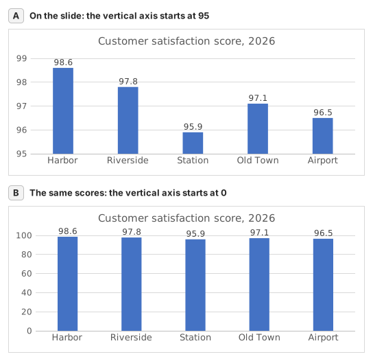
Two column charts titled "Customer satisfaction score, 2026" with the same five store scores, each column labelled: Harbor 98.6, Riverside 97.8, Station 95.9, Old Town 97.1, Airport 96.5. Chart A, as on the slide, has a vertical axis from 95 to 99, so each column shows only the part of the score above 95: Harbor's column towers over Station's. Chart B has a vertical axis from 0 to 100, and the five columns look almost the same height.
  1. Frage 1. On the slide (chart A), Harbor's column towers over Station's. How much higher is Harbor's score really? Use your column C.

    Antwort: About 3% higher

    Harbor scores 98.6 and Station 95.9, so Harbor is 98.6 ÷ 95.9 − 1 ≈ 2.8% higher. On the slide each column only shows the part above 95: 3.6 points against 0.9, which draws Harbor's column 4.0 times as tall.

  2. Frage 2. You select the slide's vertical axis and open Format Axis (right-click the axis → Format Axis). Which change makes the columns honest?

    Antwort: Type 0 in the Minimum box

    Columns show a value by their length from the axis, so the axis must start at 0 for the lengths to compare. Reset is not enough: when every value is above about five sixths of the largest one, as here, Excel's automatic minimum is not 0 either. Data labels print the true numbers but leave the misleading lengths.

  3. Frage 3. In which of these charts is a value axis that does not start at 0 acceptable? Select all that apply.

    Antworten: A line chart of a share price moving between $95 and $99 und A scatter chart of house size against sale price

    Columns and bars show a value by their length, so a cut axis turns small gaps into big ones. Lines and dots show a value by its position, so their axis may zoom into the range where the values move, as long as its labels show where it starts.

Häufige Fehler

Filling =B2/MIN(B2:B6)-1 down without $: in the rows below Station the MIN range no longer includes Station's score, so those stores are measured against the wrong lowest store.

So bewerten wir

Jede Formel, die das richtige Ergebnis liefert, wird akzeptiert, außer die Aufgabe nennt eine Funktion: Dann bringt eine andere Funktion die halbe Punktzahl. Wir vergleichen Werte mit einer kleinen Toleranz und ignorieren bei Text Groß- und Kleinschreibung sowie Leerzeichen. Eine richtige Zahl, die statt einer Formel von Hand eingetippt wurde, bringt die halbe Punktzahl. Aufgaben mit mehreren Zellen bringen die volle Punktzahl, wenn 100% der Zellen stimmen, und die halbe ab 50%. Wo es darauf ankommt, ändern wir außerdem eine Eingabezelle in einer Kopie Ihrer Tabelle und prüfen, ob Ihre Formel mitzieht.

Antworten nach den Regeln von Excel 365 berechnet und am 20. November 2026 in unserem Bewertungssystem geprüft. Verfasst von GridBelt team.

Ähnliche Übungen

  • Read a clustered column chart of revenue by regionAnfänger, ~6 Min.
  • Year-over-year % changeAnfänger, ~4 Min.
  • Revenue and margin % in one readable chartExperten, ~9 Min.

Funktionsreferenz

Offizielle Dokumentation

Nächste Übung

Series or categories? Read a chart both ways and flip its table