Zum Inhalt springen
GridBelt
  • Excel-Test
  • Übungen
  • Programme
  • Preise
Anmelden
Kostenlosen Test starten
  • Excel-Test
  • Übungen
  • Programme
  • Preise
AnmeldenKonto erstellen
Kostenlosen Test starten
GridBelt

Excel üben – direkt im Browser.

Excel-Test

  • Stufe 1: Anfänger
  • Stufe 2: Fortgeschrittene
  • Stufe 3: Experten
  • Excel-Test in 7 Tagen
  • Bestenliste
  • Excel-Test im Bewerbungsverfahren
  • Excel-Test von Indeed

Übungen

  • Alle Übungen
  • Programme
  • Für Anfänger

Ratgeber

  • Excel-Formeln
  • Excel-Tastenkombinationen

Unternehmen

  • Über uns
  • Preise
  • So bewerten wir

© GridBelt. Alle Rechte vorbehalten.

  • Datenschutzerklärung
  • Nutzungsbedingungen
  • Rückerstattungsrichtlinie

Excel ist eine Marke der Microsoft Corporation. Indeed, TestGorilla, SHL und andere Marken sind Eigentum ihrer jeweiligen Inhaber. GridBelt ist eine unabhängige Übungsplattform, steht mit Microsoft, TestGorilla, SHL oder Indeed in keiner Verbindung und wird von keinem dieser Unternehmen unterstützt oder gesponsert.

  1. Übungen
  2. /
  3. Charts

Excel chart practice: series, categories and a flipped table

  • Fortgeschrittene
  • ~7 Min.
  • Charts

Übungstext auf Englisch

An outdoor-footwear brand tracks the 2026 unit sales of three of its shoe models in A1:E4, quarter by quarter: models down the rows, quarters across. The analyst's two clustered column charts of that range are shown below. The planning sheet also needs the same numbers the other way round, quarters down the rows, as a live formula, with a total for each quarter.

Two clustered column charts titled "Units sold, 2026" drawn from the same table of three models by four quarters: Trail runner Q1 1,240, Q2 1,315, Q3 1,402, Q4 1,488; City sneaker Q1 2,210, Q2 2,050, Q3 2,390, Q4 2,275; Hiking boot Q1 980, Q2 1,105, Q3 860, Q4 1,490. The upper chart, A, has Q1 to Q4 along the horizontal axis and, in each quarter, one column per model; the legend lists Trail runner, City sneaker, Hiking boot. The lower chart, B, has the models along the horizontal axis and, for each model, one column per quarter; the legend lists Q1 to Q4.

Ihre Aufgabe

  1. 1Click G1, type =TRANSPOSE(A1:E4) and press Enter. The result spills into G1:J5: the corner label and the quarters run down column G, the models across row 1. Keep G1:J5 empty, or the formula shows #SPILL!. (Excel 2019 and older: select G1:J5 first, type the formula and confirm it as an array formula with Ctrl+Shift+Enter on Windows or ⌘+Shift+Return on a Mac.)
  2. 2The flipped copy is linked to A1:E4: when a number there changes, G1:J5 changes with it, unlike a copy made with Paste Special → Transpose.
  3. 3In K2, add up the quarter in row 2 of the flipped table: a SUM over H2:J2, its three model cells. Fill K2 down to K5 (double-click the fill handle, or select K2:K5 and press Ctrl+D / ⌘D).
  4. 4Then answer the questions about the two charts. They are pictures: this practice grid has no chart command.

Antwortzellen

Fragen

Wählen Sie hier Ihre Antworten. „Prüfen“ bewertet sie zusammen mit den Antwortzellen.

  1. Frage 1Chart A was inserted from A1:E4 with Excel's default settings. What did Excel make its data series?

    Wählen Sie eine Antwort.

  2. Frage 2Chart B shows the same cells A1:E4 as chart A. Which command turns chart A into chart B?

    Wählen Sie eine Antwort.

  3. Frage 3The sales director asks: "Did each model sell more in every quarter than in the one before?" Which chart answers that at a glance?

    Wählen Sie eine Antwort.

  4. Frage 4You insert a clustered column chart from your flipped table G1:J5 (quarters in the rows, models across) with the default settings. What does Excel put along the horizontal axis?

    Wählen Sie eine Antwort.

Feedback

Beantworten Sie die Fragen, geben Sie Ihre Formel in die Tabelle ein, drücken Sie Enter und dann „Prüfen“. Wir bewerten Ihre Antworten, den Wert in jeder Antwortzelle und die Formel dahinter.

Aufgaben

  1. Nicht geprüftIn G1, flip the table A1:E4 with one TRANSPOSE formula, labels included, so the quarters run down the rows and the models across (the result spills into G1:J5).
  2. Nicht geprüftIn K2:K5, total each quarter's units across the three models of your flipped table, with one formula filled down.
  3. Nicht geprüftFrage 1: Chart A was inserted from A1:E4 with Excel's default settings. What did Excel make its data series?
  4. Nicht geprüftFrage 2: Chart B shows the same cells A1:E4 as chart A. Which command turns chart A into chart B?
  5. Nicht geprüftFrage 3: The sales director asks: "Did each model sell more in every quarter than in the one before?" Which chart answers that at a glance?
  6. Nicht geprüftFrage 4: You insert a clustered column chart from your flipped table G1:J5 (quarters in the rows, models across) with the default settings. What does Excel put along the horizontal axis?

Für Tabellenaufgaben empfehlen wir einen Computer. Die Tabelle scrollt innerhalb dieses Rahmens.

StartInsertFormulasDataView
A1fxIhre Arbeitsmappe wird vorbereitet…
A
B
C
D
E
F
G
H
I
J
1
2
3
4
5
6
7
8
9
10
11
12
13
14
15
16
17
18
19
20
21
22
Sheet1

Beantworten Sie die Fragen, füllen Sie die Zellen aus und prüfen Sie.

Über diese Übung

Ein Datensatz mit 3 Zeilen auf einem Tabellenblatt, 2 Antwortzellen, etwa 7 Minuten. Bewertet in Ihrem Browser: der Wert und die Formel dahinter, mit Feedback, das die Korrektur benennt. Dazu kommen 4 Multiple-Choice-Fragen, die ebenfalls mit „Prüfen“ bewertet werden.

So lösen Sie die Aufgabe

  • G1=TRANSPOSE(A1:E4)
  • K2=SUM(H2:J2)

TRANSPOSE returns the table with its rows and columns swapped: =TRANSPOSE(A1:E4) puts the quarters down column G and the models across row 1, and because it is a formula the copy follows every change in A1:E4. Each quarter then sits in one row, so its total is a plain SUM across that row. The charts: Excel made the models the series of chart A because the range has fewer models than quarters; Chart Design → Switch Row/Column turns it into chart B without touching the cells; chart B puts each model's four quarters side by side, which answers "did it grow every quarter?"; and a chart of the flipped table again gets the quarters along the axis, because Excel puts the larger number of items there.

Where it lives: select the chart, then Chart Design → Data group → Switch Row/Column (in Excel 2016–2019 the tab is called Design, under Chart Tools); Chart Design → Select Data opens the same switch together with the series and category ranges, which is where you fix a chart whose series are wrong. Excel's rule (Microsoft Support): it compares the rows and columns of the selected range and puts the larger number along the horizontal axis; with as many rows as columns, each row becomes a series. Pitfall 1: Paste Special → Transpose makes a static copy that does not follow later changes, while TRANSPOSE stays linked. Pitfall 2: an empty corner cell comes out as 0 in Excel's TRANSPOSE result; a label such as Units in A1 avoids that. Pitfall 3: in Excel 2019 and older, TRANSPOSE is a legacy array formula over a selected block (Ctrl+Shift+Enter) that you can only edit or delete as a whole; in Excel 365 it spills from one cell.

Andere Wege, die funktionieren

  • =TRANSPOSE($A$1:$E$4) in G1 — the same; the $ signs make no difference to a single formula
  • =H2+I2+J2 in K2 — the same total as =SUM(H2:J2), filled down
  • =SUM(B2:B4) in K2, =SUM(C2:C4) in K3 and so on — the totals straight from the original table, one formula per quarter (it cannot be filled down)

Antworten auf die Fragen
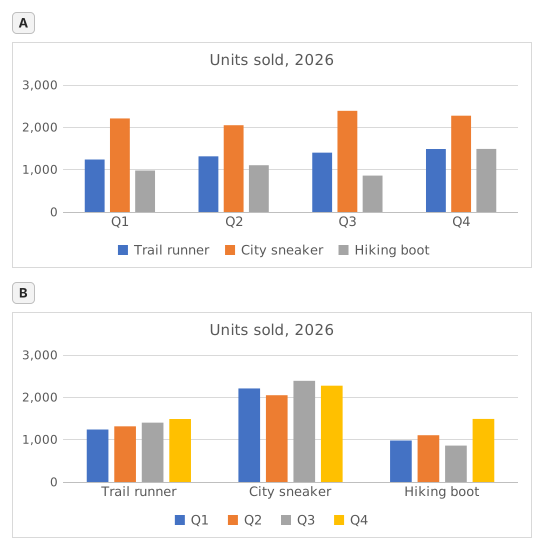
Two clustered column charts titled "Units sold, 2026" drawn from the same table of three models by four quarters: Trail runner Q1 1,240, Q2 1,315, Q3 1,402, Q4 1,488; City sneaker Q1 2,210, Q2 2,050, Q3 2,390, Q4 2,275; Hiking boot Q1 980, Q2 1,105, Q3 860, Q4 1,490. The upper chart, A, has Q1 to Q4 along the horizontal axis and, in each quarter, one column per model; the legend lists Trail runner, City sneaker, Hiking boot. The lower chart, B, has the models along the horizontal axis and, for each model, one column per quarter; the legend lists Q1 to Q4.
  1. Frage 1. Chart A was inserted from A1:E4 with Excel's default settings. What did Excel make its data series?

    Antwort: The three shoe models

    The data series are the colours listed in the legend, one per model: Trail runner, City sneaker, Hiking boot. Excel chose them because the range has 3 model rows and 4 quarter columns: it puts the larger number of items, the 4 quarters, along the horizontal axis, so each row becomes a series.

  2. Frage 2. Chart B shows the same cells A1:E4 as chart A. Which command turns chart A into chart B?

    Antwort: Chart Design → Switch Row/Column

    Switch Row/Column (Chart Design tab, Data group) swaps what the chart reads as series and as categories; the cells on the sheet stay exactly as they are. Paste Special → Transpose copies cells and leaves the chart alone, Change Chart Type changes the kind of chart, and Categories in reverse order only flips the order along the axis.

  3. Frage 3. The sales director asks: "Did each model sell more in every quarter than in the one before?" Which chart answers that at a glance?

    Antwort: Chart B

    Excel draws the series of one category side by side, and neighbouring columns are the easiest to compare. In chart B each model is a category, so its four quarters stand next to each other and a steady rise shows as a staircase (Trail runner); in chart A you would have to follow one colour across four clusters. Same numbers, different comparisons made easy.

  4. Frage 4. You insert a clustered column chart from your flipped table G1:J5 (quarters in the rows, models across) with the default settings. What does Excel put along the horizontal axis?

    Antwort: The four quarters

    Excel counts the rows and the columns of the range and puts the larger number of items along the horizontal axis: 4 quarters against 3 models, whichever way round the table is. So the flipped table gives the layout of chart A again; for the other layout, use Switch Row/Column on either chart.

Häufige Fehler

Flipping only the numbers with =TRANSPOSE(B2:E4): the labels are lost and the block lands one row and one column off, so the flipped table and the quarter totals no longer line up with the quarters.

So bewerten wir

Jede Formel, die das richtige Ergebnis liefert, wird akzeptiert, außer die Aufgabe nennt eine Funktion: Dann bringt eine andere Funktion die halbe Punktzahl. Wir vergleichen Werte mit einer kleinen Toleranz und ignorieren bei Text Groß- und Kleinschreibung sowie Leerzeichen. Eine richtige Zahl, die statt einer Formel von Hand eingetippt wurde, bringt die halbe Punktzahl. Aufgaben mit mehreren Zellen bringen die volle Punktzahl, wenn 100% der Zellen stimmen, und die halbe ab 50%. Wo es darauf ankommt, ändern wir außerdem eine Eingabezelle in einer Kopie Ihrer Tabelle und prüfen, ob Ihre Formel mitzieht.

Antworten nach den Regeln von Excel 365 berechnet und am 20. November 2026 in unserem Bewertungssystem geprüft. Verfasst von GridBelt team.

In diesen Programmen

  • Excel test in 7 days, Plan für Stufe 1Tag 6
  • Excel test in 7 days, Plan für Stufe 2Tag 5
  • Excel for Sales and MarketingTag 7

Ähnliche Übungen

  • Read a clustered column chart of revenue by regionAnfänger, ~6 Min.
  • Sales by region and product with SUMIFSFortgeschrittene, ~7 Min.
  • Pick the right chart for each questionAnfänger, ~9 Min.

Funktionsreferenz

Offizielle Dokumentation

Nächste Übung

Revenue and margin % in one readable chart