Über diese Übung
Ein Datensatz mit 150 Zeilen auf einem Tabellenblatt, 3 Antwortzellen, etwa 12 Minuten. Bewertet in Ihrem Browser: der Wert und die Formel dahinter, mit Feedback, das die Korrektur benennt. Dazu kommen 4 Multiple-Choice-Fragen, die ebenfalls mit „Prüfen“ bewertet werden.
So lösen Sie die Aufgabe
- G2
=IF(F2="",0,VALUE(F2)) - J2
=SUMPRODUCT(--ISTEXT(F2:F151)) - J3
=SUM(G2:G151)
Excel sums a value field only when every cell of it is a number. Here some amounts are text (they sit at the left of the cell) and some are blank, so the PivotTable fell back to Count of Amount, which counts every non-empty cell like COUNTA. Picking Sum without cleaning adds the text amounts as 0, so the totals come out too low: convert them first (column G), then summarize by Sum. Department belongs in Rows for one row per department, and rows pasted below a fixed source range stay outside it until you change the data source, or use an Excel Table, which grows with the data.
In desktop Excel you can fix column F in place instead of using a helper column: select F2:F151 and use the warning button next to the green triangles → Convert to Number, or Data → Text to Columns → Finish, or copy a cell that holds 1 and use Paste Special → Multiply. VALUE reads text with your own regional settings; if your Excel uses a comma as the decimal separator, =NUMBERVALUE(F2,".") reads these dot-decimal amounts correctly. Blanks: fill them with 0 (Home → Find & Select → Go To Special → Blanks, type 0, Ctrl+Enter) or keep them and pick Sum yourself. A formula that returns "" for an empty amount returns text, which keeps the field on Count. Then refresh (PivotTable Analyze → Refresh, Alt+F5 on Windows; the tab is called Analyze in Excel 2016 and 2019) and set the field to Sum: right-click a value → Summarize Values By → Sum, or Value Field Settings. Change Data Source sits on the same tab; an Excel Table (Insert → Table) grows with every row added below it, so the PivotTable picks new rows up at the next Refresh. Auto Refresh, which Microsoft lists as a Microsoft 365 Insider feature for now, refreshes PivotTables on workbook data by itself, but it never stretches a fixed range either. This in-browser grid has no PivotTable: the pictures show what Excel does, and your formulas are graded in the grid.
Andere Wege, die funktionieren
- =F2*1 or =--F2 in G2 — arithmetic turns text into a number and an empty cell into 0
- =COUNTIF(F2:F151,"*") or =COUNTA(F2:F151)-COUNT(F2:F151) in J2 — other ways to count the text cells
- =SUMPRODUCT(--F2:F151) in J3 — the clean total in one formula, without column G
Antworten auf die Fragen
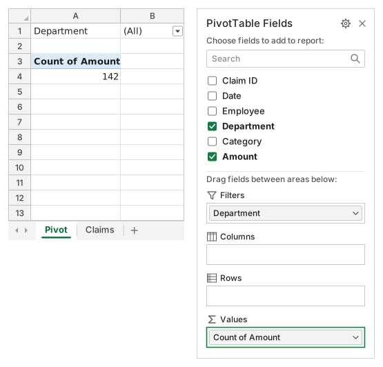
Frage 1. Which of these make Excel summarize Amount as Count instead of Sum when the field is dropped into Values? Select all that apply.
Antworten: Some amounts are stored as text und Some amount cells are blank
Excel sums a value field only when every cell of it holds a number; text that looks like a number or an empty cell makes it fall back to Count, which counts non-empty cells like COUNTA (142 of the 150 claims here). Where Department sits, decimals and refreshing play no part in that choice.
Frage 2. Suppose you change nothing in the data and only pick Sum in Value Field Settings, as pictured. What will Sum of Amount show?
Antwort: Too little: the text amounts are added as 0
A PivotTable adds only real numbers: blank or nonnumeric values become 0 when the field is summed. The text amounts drop out of every total without any warning, so convert them first (your column G) and then summarize by Sum.
Frage 3. A week later, 12 new claims are pasted below the list, in rows 152 to 163 (pictured). After Refresh the report still leaves them out. Which of these make the report include them? Select all that apply.
Antworten: Change Data Source so the range ends at row 163 und Make the claims an Excel Table and use it as the source
The PivotTable reads the fixed range Claims!$A$1:$F$151, and Refresh or Refresh All re-reads exactly that range. Change Data Source extends it once; an Excel Table (Insert → Table, Ctrl+T on Windows, ⌘T on a Mac) grows with every row added below it, so each later Refresh picks new claims up.
Frage 4. To list one row per department with its total, where should Department go in the Fields pane?
Antwort: Drag it to the Rows area
A field in Rows gives each of its items its own line, here one per department with the amounts summed beside it and a Grand Total at the bottom. Columns would spread the departments across the top, Values would count them, and a report filter shows one total at a time.
Häufige Fehler
Picking Sum in Value Field Settings without cleaning the data: the text amounts are then added as 0 and every department total is too low. Converting with =IF(F2="","",VALUE(F2)) is the other trap: its "" results are text and keep the field on Count.
So bewerten wir
Jede Formel, die das richtige Ergebnis liefert, wird akzeptiert, außer die Aufgabe nennt eine Funktion: Dann bringt eine andere Funktion die halbe Punktzahl. Wir vergleichen Werte mit einer kleinen Toleranz und ignorieren bei Text Groß- und Kleinschreibung sowie Leerzeichen. Eine richtige Zahl, die statt einer Formel von Hand eingetippt wurde, bringt die halbe Punktzahl. Aufgaben mit mehreren Zellen bringen die volle Punktzahl, wenn 100% der Zellen stimmen, und die halbe ab 50%. Wo es darauf ankommt, ändern wir außerdem eine Eingabezelle in einer Kopie Ihrer Tabelle und prüfen, ob Ihre Formel mitzieht.
Antworten nach den Regeln von Excel 365 berechnet und am 20. November 2026 in unserem Bewertungssystem geprüft. Verfasst von GridBelt team.