Über diese Übung
Ein Datensatz mit 210 Zeilen auf einem Tabellenblatt, 2 Antwortzellen, etwa 8 Minuten. Bewertet in Ihrem Browser: der Wert und die Formel dahinter, mit Feedback, das die Korrektur benennt. Dazu kommen 4 Multiple-Choice-Fragen, die ebenfalls mit „Prüfen“ bewertet werden.
So lösen Sie die Aufgabe
- I4
=SUMIFS(F2:F211,C2:C211,I2,D2:D211,I3) - I5
=AVERAGEIFS(F2:F211,C2:C211,I2,D2:D211,I3)
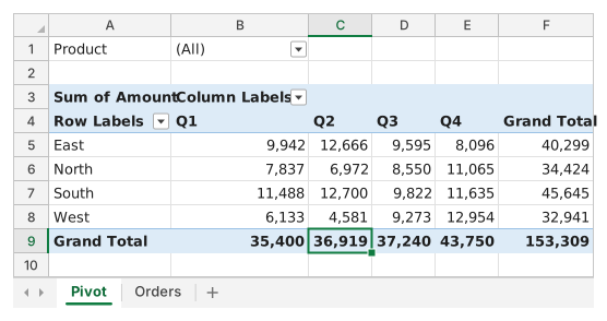
A PivotTable value cell is a SUMIFS in disguise: it adds the Amount of the orders whose Region matches its row and whose Quarter matches its column, so =SUMIFS(F2:F211,C2:C211,I2,D2:D211,I3) reproduces the East / Q3 cell exactly, and AVERAGEIFS gives the average the report leaves out. Reading the report: the field in Columns (Quarter) makes the headings across the top and the field in Rows (Region) the labels down the side; the Grand Total row adds each column down (C9 is Q2 for all regions), the Grand Total column adds each row across, and F9 is the year. South leads the year although West has the biggest single quarter, and double-clicking any value cell lists the orders behind it.
Where it lives in Excel: Insert → PivotTable builds the report; the PivotTable Fields pane opens whenever a report cell is selected (PivotTable Analyze → Field List brings it back; the tab is called Analyze in Excel 2016 and 2019). Show Details: double-click a value or right-click → Show Details, and the rows behind it land on a new sheet (PivotTable Options → Data → Enable show details switches this off). To show averages in the report itself, add Amount to Values a second time and set Value Field Settings → Summarize value field by → Average. Pitfall 1: the report is a snapshot of the source; after the orders change, click Refresh (PivotTable Analyze → Refresh, Alt+F5 on Windows). Auto Refresh, which Microsoft lists as a Microsoft 365 Insider feature for now, updates PivotTables on workbook data by itself; without it the report waits for Refresh. Pitfall 2: clicking a report cell while you type a formula inserts a GETPIVOTDATA formula such as =GETPIVOTDATA("Amount",Pivot!$A$3,"Region","East","Quarter","Q3") instead of a plain reference; it keeps pointing at the right number when the report changes shape, and PivotTable Analyze → Options → Generate GetPivotData turns it off. Pitfall 3: the biggest number in the grid is a single cell, not the best region; compare the Grand Total column. This in-browser grid has no PivotTable: the report is a picture drawn from the same 210 orders, and your SUMIFS and AVERAGEIFS formulas are graded in the grid.
Andere Wege, die funktionieren
- =SUMPRODUCT((C2:C211=I2)*(D2:D211=I3)*F2:F211) — the array form of the same sum
- =I4/COUNTIFS(C2:C211,I2,D2:D211,I3) — the average as the sum divided by the number of orders
- =AVERAGE(FILTER(F2:F211,(C2:C211=I2)*(D2:D211=I3))) — Excel 365 only
Antworten auf die Fragen
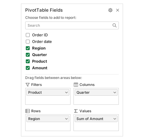
Frage 1. Look at the Fields pane: which part of the report does the field in its Columns area produce?
Antwort: The Q1 to Q4 headings across the top
Quarter sits in the Columns area, and a field in Columns turns its items into the headings across the top of the report. Region in Rows gives the labels down the side, Amount in Values the numbers, and Product in Filters the (All) box above.
Frage 2. What does the number in C9 of the Pivot sheet, where the Grand Total row meets the Q2 column, show?
Antwort: The Q2 amount of all four regions added together
The Grand Total row adds each column down: C9 = 12,666 + 6,972 + 12,700 + 4,581 = 36,919. The whole year of every region is the bottom-right cell F9, and a number of orders would need Count instead of Sum.
Frage 3. Which region brought in the largest amount over the whole year?
Antwort: South
Read the Grand Total column (F5:F8): South has the largest year, 45,645. West owns the biggest single number in the report (12,954 in Q4) but its year adds up to only 32,941.
Frage 4. You want to see the individual orders behind the East / Q3 number. What is the quickest way in Excel?
Antwort: Double-click that value cell
Double-clicking a value cell (or right-click → Show Details) puts the orders behind that number on a new worksheet. Refresh only re-reads the source data, Order ID in Values would count the orders, and PivotTable cells hold no formula to open.
Häufige Fehler
Typing the criteria into the formula, =SUMIFS(F2:F211,C2:C211,"East",D2:D211,"Q3"): the value matches today, but the checker switches I2 and I3 and the hard-coded formula does not follow.
So bewerten wir
Jede Formel, die das richtige Ergebnis liefert, wird akzeptiert, außer die Aufgabe nennt eine Funktion: Dann bringt eine andere Funktion die halbe Punktzahl. Wir vergleichen Werte mit einer kleinen Toleranz und ignorieren bei Text Groß- und Kleinschreibung sowie Leerzeichen. Eine richtige Zahl, die statt einer Formel von Hand eingetippt wurde, bringt die halbe Punktzahl. Aufgaben mit mehreren Zellen bringen die volle Punktzahl, wenn 100% der Zellen stimmen, und die halbe ab 50%. Wo es darauf ankommt, ändern wir außerdem eine Eingabezelle in einer Kopie Ihrer Tabelle und prüfen, ob Ihre Formel mitzieht.
Antworten nach den Regeln von Excel 365 berechnet und am 20. November 2026 in unserem Bewertungssystem geprüft. Verfasst von GridBelt team.