Saltar al contenido
GridBelt
  • Prueba de Excel
  • Práctica
  • Programas
  • Precios
Iniciar sesión
Empezar la prueba gratuita
  • Prueba de Excel
  • Práctica
  • Programas
  • Precios
Iniciar sesiónCrear cuenta
Empezar la prueba gratuita
GridBelt

Practica Excel en tu navegador.

Prueba de Excel

  • Nivel 1: Principiante
  • Nivel 2: Intermedio
  • Nivel 3: Experto
  • Prueba de Excel en 7 días
  • Clasificación
  • Prueba de Excel para entrevistas
  • Evaluación de Excel de Indeed

Práctica

  • Todos los ejercicios
  • Programas
  • Para principiantes

Guías

  • Fórmulas de Excel
  • Atajos de Excel

Empresa

  • Acerca de
  • Precios
  • Cómo corregimos

© GridBelt. Todos los derechos reservados.

  • Política de privacidad
  • Términos de uso
  • Política de reembolso

Excel es una marca comercial de Microsoft Corporation. Indeed, TestGorilla, SHL y otras marcas son propiedad de sus respectivos titulares. GridBelt es un sitio de práctica independiente y no está afiliado a Microsoft, TestGorilla, SHL ni Indeed, ni respaldado ni patrocinado por ellos.

  1. Práctica
  2. /
  3. Charts

Excel chart practice: spot a misleading axis that does not start at zero

  • Intermedio
  • ~8 min
  • Charts

Enunciado en inglés

A home-improvement chain surveys its customers every month. The regional manager's slide shows the 2026 satisfaction scores (0 to 100) of five stores as columns on a vertical axis that starts at 95, and one store looks far ahead of the rest; the manager wants to reward it. Before the meeting, measure the real difference in the sheet: the scores are in A1:B6 and the slide's axis minimum is in F2.

Two column charts titled "Customer satisfaction score, 2026" with the same five store scores, each column labelled: Harbor 98.6, Riverside 97.8, Station 95.9, Old Town 97.1, Airport 96.5. Chart A, as on the slide, has a vertical axis from 95 to 99, so each column shows only the part of the score above 95: Harbor's column towers over Station's. Chart B has a vertical axis from 0 to 100, and the five columns look almost the same height.

Qué tienes que hacer

  1. 1Click C2 and compare the store with the lowest score of all five: divide B2 by MIN($B$2:$B$6) and subtract 1. The $ signs keep MIN on all five stores when you fill down — F4 (Windows) or ⌘T (Mac) adds them.
  2. 2Fill C2 down to C6, then format C2:C6 as a percentage with one decimal place: Ctrl+Shift+% (Control+Shift+% on a Mac), then Increase Decimal once (in this grid: the toolbar's Increase decimal places button, under ⋮ when the toolbar is narrow; in Excel, Format Cells with Ctrl+1 / ⌘1 → Percentage → 1 decimal place works too). The lowest store shows 0.0%.
  3. 3On a chart, a column is drawn from the axis minimum up to its value, so its drawn height is the value minus the minimum. In F3, divide the drawn height of the tallest column by that of the shortest: (MAX(B2:B6) − F2) ÷ (MIN(B2:B6) − F2). Refer to F2 and do not type the minimum into the formula, so that F3 still works when the axis minimum changes.
  4. 4Then answer the questions; the charts are pictures, because this practice grid has no chart command.

Celdas de respuesta

Preguntas

Elige aquí tus respuestas: el botón Comprobar las corrige junto con las celdas de respuesta.

  1. Pregunta 1On the slide (chart A), Harbor's column towers over Station's. How much higher is Harbor's score really? Use your column C.

    Elige una respuesta.

  2. Pregunta 2You select the slide's vertical axis and open Format Axis (right-click the axis → Format Axis). Which change makes the columns honest?

    Elige una respuesta.

    The slide's column chart "Customer satisfaction score, 2026", narrower here, with the store names slanted; its vertical axis (95 to 99) is selected, and the Format Axis pane is open at Axis Options. Under Bounds, Minimum shows 95.0 with a Reset button next to it and Maximum shows 99.0 with an Auto button; under Units, Major shows 1.0 and Minor 0.2, both Auto.
  3. Pregunta 3In which of these charts is a value axis that does not start at 0 acceptable? Select all that apply.

    Selecciona todas las que correspondan.

Corrección

Responde a las preguntas, escribe tu fórmula en la cuadrícula, presiona Enter y luego haz clic en Comprobar. Evaluamos tus respuestas, el valor de cada celda de respuesta y la fórmula que lo produce.

Tareas

  1. Sin comprobarIn C2:C6, compute how much higher each store's score is than the lowest of the five scores, as a share of the lowest — score ÷ lowest − 1 — with one formula filled down.
  2. Sin comprobarFormat C2:C6 as a percentage with one decimal place (0.0%, for example 1.2%).
  3. Sin comprobarIn F3, compute how many times taller the tallest column is drawn than the shortest on an axis that starts at the value in F2: (highest score − F2) ÷ (lowest score − F2).
  4. Sin comprobarPregunta 1: On the slide (chart A), Harbor's column towers over Station's. How much higher is Harbor's score really? Use your column C.
  5. Sin comprobarPregunta 2: You select the slide's vertical axis and open Format Axis (right-click the axis → Format Axis). Which change makes the columns honest?
  6. Sin comprobarPregunta 3: In which of these charts is a value axis that does not start at 0 acceptable? Select all that apply.

Para las tareas de hoja de cálculo se recomienda una pantalla grande. La hoja se desplaza dentro de este recuadro.

StartInsertFormulasDataView
A1fxPreparando tu libro…
A
B
C
D
E
F
G
H
I
J
1
2
3
4
5
6
7
8
9
10
11
12
13
14
15
16
17
18
19
20
21
22
Sheet1

Responde a las preguntas, rellena las celdas y comprueba.

Sobre este ejercicio

Un conjunto de datos de 5 filas en una hoja, 2 celdas de respuesta, unos 8 minutos. Se corrige en tu navegador: el valor y la fórmula que lo produce, con comentarios que te dicen qué arreglar. Incluye además 3 preguntas de opción múltiple, que se corrigen con el mismo botón Comprobar.

Cómo resolverlo

  • C2=B2/MIN($B$2:$B$6)-1
  • F3=(MAX(B2:B6)-F2)/(MIN(B2:B6)-F2)

Harbor's score is only 2.8% above Station's (=B2/MIN($B$2:$B$6)-1), but on an axis that starts at 95 a column only shows the part of its value above 95, so Harbor's 3.6 points against Station's 0.9 draw a column 4.0 times as tall (F3). With the axis from 0 the drawn heights are the real values and the ratio falls to 1.03. The fix is to type 0 as the axis Minimum; a non-zero axis is acceptable for lines and dots, which show values by position rather than by length.

In Excel, right-click the vertical axis → Format Axis → Axis Options → Bounds and type 0 in Minimum (the same pane on Windows and Mac, and in Excel 2016–2021). When a bound is on Auto, Excel chooses it: if the smallest value is above about five sixths of the largest, the automatic minimum is not 0, so five scores between 95.9 and 98.6 get a cut axis even if nobody set one, and Reset only returns to that automatic value. The picture shows a 300% difference where the data has 2.8%; Tufte called the ratio of the two the lie factor. When small differences matter, chart them directly: columns of each store's gap to the lowest store or to a target, a dot plot, or a line with a clearly labelled axis. Pitfall: =B2/MIN(B2:B6)-1 without $ slides the MIN range down as you fill, so the stores below Station are compared with a different "lowest" score.

Otras formas válidas

  • =B2/MIN(B$2:B$6)-1 — locking the rows is enough when you only fill down
  • =(B2-MIN($B$2:$B$6))/MIN($B$2:$B$6) — the same, written as (score − lowest) ÷ lowest
  • =(MAX(B2:B6)-$F$2)/(MIN(B2:B6)-$F$2) in F3 — the same with F2 locked

Respuestas a las preguntas
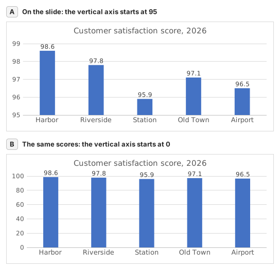
Two column charts titled "Customer satisfaction score, 2026" with the same five store scores, each column labelled: Harbor 98.6, Riverside 97.8, Station 95.9, Old Town 97.1, Airport 96.5. Chart A, as on the slide, has a vertical axis from 95 to 99, so each column shows only the part of the score above 95: Harbor's column towers over Station's. Chart B has a vertical axis from 0 to 100, and the five columns look almost the same height.
  1. Pregunta 1. On the slide (chart A), Harbor's column towers over Station's. How much higher is Harbor's score really? Use your column C.

    Respuesta: About 3% higher

    Harbor scores 98.6 and Station 95.9, so Harbor is 98.6 ÷ 95.9 − 1 ≈ 2.8% higher. On the slide each column only shows the part above 95: 3.6 points against 0.9, which draws Harbor's column 4.0 times as tall.

  2. Pregunta 2. You select the slide's vertical axis and open Format Axis (right-click the axis → Format Axis). Which change makes the columns honest?

    Respuesta: Type 0 in the Minimum box

    Columns show a value by their length from the axis, so the axis must start at 0 for the lengths to compare. Reset is not enough: when every value is above about five sixths of the largest one, as here, Excel's automatic minimum is not 0 either. Data labels print the true numbers but leave the misleading lengths.

  3. Pregunta 3. In which of these charts is a value axis that does not start at 0 acceptable? Select all that apply.

    Respuestas: A line chart of a share price moving between $95 and $99 y A scatter chart of house size against sale price

    Columns and bars show a value by their length, so a cut axis turns small gaps into big ones. Lines and dots show a value by its position, so their axis may zoom into the range where the values move, as long as its labels show where it starts.

Errores frecuentes

Filling =B2/MIN(B2:B6)-1 down without $: in the rows below Station the MIN range no longer includes Station's score, so those stores are measured against the wrong lowest store.

Cómo corregimos

Se acepta cualquier fórmula que produzca el resultado correcto, salvo que la tarea nombre una función: entonces otra función obtiene media puntuación. Comparamos los valores con una pequeña tolerancia y, en el texto, ignoramos mayúsculas y espacios. Un número correcto escrito a mano en lugar de una fórmula obtiene media puntuación. Las tareas de varias celdas obtienen la puntuación completa con el 100% de las celdas correctas y media puntuación desde el 50%. Cuando importa, también cambiamos una celda de entrada en una copia de tu hoja y comprobamos que tu fórmula se adapta.

Respuestas calculadas con las reglas de Excel 365 y comprobadas en nuestro corrector el 20 de noviembre de 2026. Autor: GridBelt team.

Ejercicios relacionados

  • Read a clustered column chart of revenue by regionPrincipiante, ~6 min
  • Year-over-year % changePrincipiante, ~4 min
  • Revenue and margin % in one readable chartExperto, ~9 min

Referencia de la función

Documentación oficial

Siguiente ejercicio

Series or categories? Read a chart both ways and flip its table