About this exercise
A 12-row dataset on one sheet, one answer cell, about 9 minutes. Graded in your browser: the value and the formula behind it, with feedback that names the fix. It also asks 4 multiple-choice questions, graded with the same Check.
How to solve it
- E2
=IFERROR(D2/B2,NA())
=IFERROR(D2/B2,NA()) divides gross profit by revenue and, for February's 0 ÷ 0, returns #N/A instead of #DIV/0!; formatted as 0.0% the margins read 44.1%, 35.2% and so on. In chart A the margins (all below 0.5) share a dollar axis built for tens of thousands, so the line looks flat; chart B moves the margin to a secondary axis with its own scale from 0% to 50%. #N/A keeps February out of the line, whereas "" would be plotted as 0%. In chart B you read the margin on the right-hand axis, the crossings of line and columns mean nothing, and the best margin (January) is not the best gross profit (July).
For an existing chart, two routes in Excel 365: right-click the margin line → Format Data Series → Series Options → Secondary Axis (Windows and Mac); or select the chart → Chart Design → Change Chart Type → Combo, set Gross margin to Line and tick its Secondary Axis box (Windows). Insert → Insert Combo Chart → Clustered Column – Line on Secondary Axis builds such a chart from scratch: select A1:B13, add E1:E13 with Ctrl (⌘ on a Mac), and the margin, the second series, becomes the line. Excel 2016–2019 for Windows work the same way; the tab is called Design, under Chart Tools. Use a secondary axis for a second unit, percent next to dollars; two dollar series belong on one axis, or readers compare heights measured against different scales. Add axis titles (Chart Design → Add Chart Element → Axis Titles) so nobody reads the margin against dollars. Charts plot "" as zero, so chart data should return NA(). #N/A never becomes a point. With Select Data → Hidden and Empty Cells → Show #N/A as an empty cell ticked (new charts in Excel 365 have it on) and empty cells shown as Gaps, the line breaks at February, as in chart B; with that box cleared, it runs straight from January to March. For a table people read, a text such as n/a is friendlier (see the IFERROR margin exercise). IFERROR also hides other errors, such as a text value in a revenue cell; =IF(B2=0,NA(),D2/B2) guards only the zero.
Other ways that work
- =IF(B2=0,NA(),D2/B2) — guards only the zero revenue and lets any other error show
- =IFERROR((B2-C2)/B2,NA()) — the margin straight from revenue and cost of sales
- =IF(ISERROR(D2/B2),NA(),D2/B2) — the pre-2007 pattern, same result
Answers to the questions
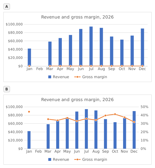
Question 1. In chart A, revenue and gross margin share one vertical axis. Why does the margin line lie flat along the bottom?
Answer: Margins below 0.5 share an axis built for dollars
On one axis every series uses the same scale: the axis runs to $100,000 for the revenue, so margins between 31.8% and 44.1% (0.32 to 0.44 as numbers) sit a hair above zero and every change disappears. The margin did move; it only needs its own scale.
Question 2. Chart B shows the same two series after one change. Which change was it?
Answer: Gross margin series → Format Data Series → Secondary Axis
Putting the margin on a secondary axis gives it its own scale on the right (0% to 50% here) while revenue keeps the dollar axis on the left. A Maximum of 1 would cut every revenue column off at the top, Display units only relabels the axis in thousands without changing the scale, and Switch Row/Column would turn the months into series.
Question 3. In chart B the margin line has no point for February, because that margin cell holds #N/A. What would the chart show if the formula returned empty text ("") for February instead?
Answer: A point at 0% for February
A formula that returns "" leaves text in the cell, not an empty cell, and Excel plots text in a line or column series as 0, so the line would dive to 0% in February. #N/A is never plotted as a point: chart B shows it as an empty cell, a gap (Select Data → Hidden and Empty Cells → Show #N/A as an empty cell), and with that box cleared the line would run straight from January to March, still without a February point.
Question 4. Which statements about chart B are true? Select all that apply.
Answers: You read the margin on the right-hand axis and Where the line crosses a column means nothing
The margin is plotted against the right-hand axis and the revenue against the left-hand one, so a point where the line meets a column only reflects how the two scales happen to be set. The highest margin, January's 44.1%, comes from a quiet month: July's 35.8% on far more revenue earned more gross profit ($33,780 against $18,440).
Common mistakes
Using =IFERROR(D2/B2,"") or =IFERROR(D2/B2,0): the table looks tidy, but a chart draws February at 0% and the margin line dives to the bottom; NA() keeps the month out of the chart.
How we grade
Any formula that produces the right result is accepted, unless the task names a function: then another function earns half credit. We compare values with a small tolerance and ignore case and spaces in text. A correct number typed by hand instead of a formula earns half credit. Multi-cell tasks earn full credit at 100% of cells, half credit from 50%. Where it matters, we also change an input cell on a copy of your sheet and check that your formula follows.
Answers computed with Excel 365 rules and checked in our grading engine on November 20, 2026. Author: GridBelt team.