Skip to content
GridBelt
  • Excel Test
  • Practice
  • Programs
  • Pricing
Sign in
Start the free test
  • Excel Test
  • Practice
  • Programs
  • Pricing
Sign inCreate account
Start the free test
GridBelt

Practice Excel in your browser.

Excel Test

  • Level 1: Beginner
  • Level 2: Intermediate
  • Level 3: Expert
  • Excel test in 7 days
  • Leaderboard
  • Excel test for interview
  • Indeed Excel assessment

Practice

  • All exercises
  • Programs
  • For beginners

Guides

  • Excel formulas
  • Excel shortcuts

Company

  • About
  • Pricing
  • How we grade

© GridBelt. All rights reserved.

  • Privacy Policy
  • Terms of Use
  • Refund Policy

Excel is a trademark of Microsoft Corporation. Indeed, TestGorilla, SHL and other marks are the property of their owners. GridBelt is an independent practice site and is not affiliated with, endorsed by or sponsored by Microsoft, TestGorilla, SHL or Indeed.

  1. Practice
  2. /
  3. Charts

Excel chart practice: spot a misleading axis that does not start at zero

  • Intermediate
  • ~8 min
  • Charts

A home-improvement chain surveys its customers every month. The regional manager's slide shows the 2026 satisfaction scores (0 to 100) of five stores as columns on a vertical axis that starts at 95, and one store looks far ahead of the rest; the manager wants to reward it. Before the meeting, measure the real difference in the sheet: the scores are in A1:B6 and the slide's axis minimum is in F2.

Two column charts titled "Customer satisfaction score, 2026" with the same five store scores, each column labelled: Harbor 98.6, Riverside 97.8, Station 95.9, Old Town 97.1, Airport 96.5. Chart A, as on the slide, has a vertical axis from 95 to 99, so each column shows only the part of the score above 95: Harbor's column towers over Station's. Chart B has a vertical axis from 0 to 100, and the five columns look almost the same height.

What you need to do

  1. 1Click C2 and compare the store with the lowest score of all five: divide B2 by MIN($B$2:$B$6) and subtract 1. The $ signs keep MIN on all five stores when you fill down — F4 (Windows) or ⌘T (Mac) adds them.
  2. 2Fill C2 down to C6, then format C2:C6 as a percentage with one decimal place: Ctrl+Shift+% (Control+Shift+% on a Mac), then Increase Decimal once (in this grid: the toolbar's Increase decimal places button, under ⋮ when the toolbar is narrow; in Excel, Format Cells with Ctrl+1 / ⌘1 → Percentage → 1 decimal place works too). The lowest store shows 0.0%.
  3. 3On a chart, a column is drawn from the axis minimum up to its value, so its drawn height is the value minus the minimum. In F3, divide the drawn height of the tallest column by that of the shortest: (MAX(B2:B6) − F2) ÷ (MIN(B2:B6) − F2). Refer to F2 and do not type the minimum into the formula, so that F3 still works when the axis minimum changes.
  4. 4Then answer the questions; the charts are pictures, because this practice grid has no chart command.

Answer cells

Questions

Pick your answers here. Check grades them together with the answer cells.

  1. Question 1On the slide (chart A), Harbor's column towers over Station's. How much higher is Harbor's score really? Use your column C.

    Choose one answer.

  2. Question 2You select the slide's vertical axis and open Format Axis (right-click the axis → Format Axis). Which change makes the columns honest?

    Choose one answer.

    The slide's column chart "Customer satisfaction score, 2026", narrower here, with the store names slanted; its vertical axis (95 to 99) is selected, and the Format Axis pane is open at Axis Options. Under Bounds, Minimum shows 95.0 with a Reset button next to it and Maximum shows 99.0 with an Auto button; under Units, Major shows 1.0 and Minor 0.2, both Auto.
  3. Question 3In which of these charts is a value axis that does not start at 0 acceptable? Select all that apply.

Feedback

Answer the questions and type your formula in the grid (press Enter), then Check. We grade your answers, the value in each answer cell and the formula behind it.

Tasks

  1. Not checkedIn C2:C6, compute how much higher each store's score is than the lowest of the five scores, as a share of the lowest — score ÷ lowest − 1 — with one formula filled down.
  2. Not checkedFormat C2:C6 as a percentage with one decimal place (0.0%, for example 1.2%).
  3. Not checkedIn F3, compute how many times taller the tallest column is drawn than the shortest on an axis that starts at the value in F2: (highest score − F2) ÷ (lowest score − F2).
  4. Not checkedQuestion 1: On the slide (chart A), Harbor's column towers over Station's. How much higher is Harbor's score really? Use your column C.
  5. Not checkedQuestion 2: You select the slide's vertical axis and open Format Axis (right-click the axis → Format Axis). Which change makes the columns honest?
  6. Not checkedQuestion 3: In which of these charts is a value axis that does not start at 0 acceptable? Select all that apply.

Desktop recommended for spreadsheet tasks. The sheet scrolls inside this box.

StartInsertFormulasDataView
A1fxPreparing your workbook…
A
B
C
D
E
F
G
H
I
J
1
2
3
4
5
6
7
8
9
10
11
12
13
14
15
16
17
18
19
20
21
22
Sheet1

Answer the questions, fill the cells, then check.

About this exercise

A 5-row dataset on one sheet, 2 answer cells, about 8 minutes. Graded in your browser: the value and the formula behind it, with feedback that names the fix. It also asks 3 multiple-choice questions, graded with the same Check.

How to solve it

  • C2=B2/MIN($B$2:$B$6)-1
  • F3=(MAX(B2:B6)-F2)/(MIN(B2:B6)-F2)

Harbor's score is only 2.8% above Station's (=B2/MIN($B$2:$B$6)-1), but on an axis that starts at 95 a column only shows the part of its value above 95, so Harbor's 3.6 points against Station's 0.9 draw a column 4.0 times as tall (F3). With the axis from 0 the drawn heights are the real values and the ratio falls to 1.03. The fix is to type 0 as the axis Minimum; a non-zero axis is acceptable for lines and dots, which show values by position rather than by length.

In Excel, right-click the vertical axis → Format Axis → Axis Options → Bounds and type 0 in Minimum (the same pane on Windows and Mac, and in Excel 2016–2021). When a bound is on Auto, Excel chooses it: if the smallest value is above about five sixths of the largest, the automatic minimum is not 0, so five scores between 95.9 and 98.6 get a cut axis even if nobody set one, and Reset only returns to that automatic value. The picture shows a 300% difference where the data has 2.8%; Tufte called the ratio of the two the lie factor. When small differences matter, chart them directly: columns of each store's gap to the lowest store or to a target, a dot plot, or a line with a clearly labelled axis. Pitfall: =B2/MIN(B2:B6)-1 without $ slides the MIN range down as you fill, so the stores below Station are compared with a different "lowest" score.

Other ways that work

  • =B2/MIN(B$2:B$6)-1 — locking the rows is enough when you only fill down
  • =(B2-MIN($B$2:$B$6))/MIN($B$2:$B$6) — the same, written as (score − lowest) ÷ lowest
  • =(MAX(B2:B6)-$F$2)/(MIN(B2:B6)-$F$2) in F3 — the same with F2 locked

Answers to the questions
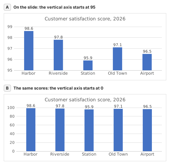
Two column charts titled "Customer satisfaction score, 2026" with the same five store scores, each column labelled: Harbor 98.6, Riverside 97.8, Station 95.9, Old Town 97.1, Airport 96.5. Chart A, as on the slide, has a vertical axis from 95 to 99, so each column shows only the part of the score above 95: Harbor's column towers over Station's. Chart B has a vertical axis from 0 to 100, and the five columns look almost the same height.
  1. Question 1. On the slide (chart A), Harbor's column towers over Station's. How much higher is Harbor's score really? Use your column C.

    Answer: About 3% higher

    Harbor scores 98.6 and Station 95.9, so Harbor is 98.6 ÷ 95.9 − 1 ≈ 2.8% higher. On the slide each column only shows the part above 95: 3.6 points against 0.9, which draws Harbor's column 4.0 times as tall.

  2. Question 2. You select the slide's vertical axis and open Format Axis (right-click the axis → Format Axis). Which change makes the columns honest?

    Answer: Type 0 in the Minimum box

    Columns show a value by their length from the axis, so the axis must start at 0 for the lengths to compare. Reset is not enough: when every value is above about five sixths of the largest one, as here, Excel's automatic minimum is not 0 either. Data labels print the true numbers but leave the misleading lengths.

  3. Question 3. In which of these charts is a value axis that does not start at 0 acceptable? Select all that apply.

    Answers: A line chart of a share price moving between $95 and $99 and A scatter chart of house size against sale price

    Columns and bars show a value by their length, so a cut axis turns small gaps into big ones. Lines and dots show a value by its position, so their axis may zoom into the range where the values move, as long as its labels show where it starts.

Common mistakes

Filling =B2/MIN(B2:B6)-1 down without $: in the rows below Station the MIN range no longer includes Station's score, so those stores are measured against the wrong lowest store.

How we grade

Any formula that produces the right result is accepted, unless the task names a function: then another function earns half credit. We compare values with a small tolerance and ignore case and spaces in text. A correct number typed by hand instead of a formula earns half credit. Multi-cell tasks earn full credit at 100% of cells, half credit from 50%. Where it matters, we also change an input cell on a copy of your sheet and check that your formula follows.

Answers computed with Excel 365 rules and checked in our grading engine on November 20, 2026. Author: GridBelt team.

Related exercises

  • Read a clustered column chart of revenue by regionBeginner, ~6 min
  • Year-over-year % changeBeginner, ~4 min
  • Revenue and margin % in one readable chartExpert, ~9 min

Function reference

Official documentation

Next exercise

Series or categories? Read a chart both ways and flip its table