Skip to content
GridBelt
  • Excel Test
  • Practice
  • Programs
  • Pricing
Sign in
Start the free test
  • Excel Test
  • Practice
  • Programs
  • Pricing
Sign inCreate account
Start the free test
GridBelt

Practice Excel in your browser.

Excel Test

  • Level 1: Beginner
  • Level 2: Intermediate
  • Level 3: Expert
  • Excel test in 7 days
  • Leaderboard
  • Excel test for interview
  • Indeed Excel assessment

Practice

  • All exercises
  • Programs
  • For beginners

Guides

  • Excel formulas
  • Excel shortcuts

Company

  • About
  • Pricing
  • How we grade

© GridBelt. All rights reserved.

  • Privacy Policy
  • Terms of Use
  • Refund Policy

Excel is a trademark of Microsoft Corporation. Indeed, TestGorilla, SHL and other marks are the property of their owners. GridBelt is an independent practice site and is not affiliated with, endorsed by or sponsored by Microsoft, TestGorilla, SHL or Indeed.

  1. Practice
  2. /
  3. Charts

Excel chart practice: series, categories and a flipped table

  • Intermediate
  • ~7 min
  • Charts

An outdoor-footwear brand tracks the 2026 unit sales of three of its shoe models in A1:E4, quarter by quarter: models down the rows, quarters across. The analyst's two clustered column charts of that range are shown below. The planning sheet also needs the same numbers the other way round, quarters down the rows, as a live formula, with a total for each quarter.

Two clustered column charts titled "Units sold, 2026" drawn from the same table of three models by four quarters: Trail runner Q1 1,240, Q2 1,315, Q3 1,402, Q4 1,488; City sneaker Q1 2,210, Q2 2,050, Q3 2,390, Q4 2,275; Hiking boot Q1 980, Q2 1,105, Q3 860, Q4 1,490. The upper chart, A, has Q1 to Q4 along the horizontal axis and, in each quarter, one column per model; the legend lists Trail runner, City sneaker, Hiking boot. The lower chart, B, has the models along the horizontal axis and, for each model, one column per quarter; the legend lists Q1 to Q4.

What you need to do

  1. 1Click G1, type =TRANSPOSE(A1:E4) and press Enter. The result spills into G1:J5: the corner label and the quarters run down column G, the models across row 1. Keep G1:J5 empty, or the formula shows #SPILL!. (Excel 2019 and older: select G1:J5 first, type the formula and confirm it as an array formula with Ctrl+Shift+Enter on Windows or ⌘+Shift+Return on a Mac.)
  2. 2The flipped copy is linked to A1:E4: when a number there changes, G1:J5 changes with it, unlike a copy made with Paste Special → Transpose.
  3. 3In K2, add up the quarter in row 2 of the flipped table: a SUM over H2:J2, its three model cells. Fill K2 down to K5 (double-click the fill handle, or select K2:K5 and press Ctrl+D / ⌘D).
  4. 4Then answer the questions about the two charts. They are pictures: this practice grid has no chart command.

Answer cells

Questions

Pick your answers here. Check grades them together with the answer cells.

  1. Question 1Chart A was inserted from A1:E4 with Excel's default settings. What did Excel make its data series?

    Choose one answer.

  2. Question 2Chart B shows the same cells A1:E4 as chart A. Which command turns chart A into chart B?

    Choose one answer.

  3. Question 3The sales director asks: "Did each model sell more in every quarter than in the one before?" Which chart answers that at a glance?

    Choose one answer.

  4. Question 4You insert a clustered column chart from your flipped table G1:J5 (quarters in the rows, models across) with the default settings. What does Excel put along the horizontal axis?

    Choose one answer.

Feedback

Answer the questions and type your formula in the grid (press Enter), then Check. We grade your answers, the value in each answer cell and the formula behind it.

Tasks

  1. Not checkedIn G1, flip the table A1:E4 with one TRANSPOSE formula, labels included, so the quarters run down the rows and the models across (the result spills into G1:J5).
  2. Not checkedIn K2:K5, total each quarter's units across the three models of your flipped table, with one formula filled down.
  3. Not checkedQuestion 1: Chart A was inserted from A1:E4 with Excel's default settings. What did Excel make its data series?
  4. Not checkedQuestion 2: Chart B shows the same cells A1:E4 as chart A. Which command turns chart A into chart B?
  5. Not checkedQuestion 3: The sales director asks: "Did each model sell more in every quarter than in the one before?" Which chart answers that at a glance?
  6. Not checkedQuestion 4: You insert a clustered column chart from your flipped table G1:J5 (quarters in the rows, models across) with the default settings. What does Excel put along the horizontal axis?

Desktop recommended for spreadsheet tasks. The sheet scrolls inside this box.

StartInsertFormulasDataView
A1fxPreparing your workbook…
A
B
C
D
E
F
G
H
I
J
1
2
3
4
5
6
7
8
9
10
11
12
13
14
15
16
17
18
19
20
21
22
Sheet1

Answer the questions, fill the cells, then check.

About this exercise

A 3-row dataset on one sheet, 2 answer cells, about 7 minutes. Graded in your browser: the value and the formula behind it, with feedback that names the fix. It also asks 4 multiple-choice questions, graded with the same Check.

How to solve it

  • G1=TRANSPOSE(A1:E4)
  • K2=SUM(H2:J2)

TRANSPOSE returns the table with its rows and columns swapped: =TRANSPOSE(A1:E4) puts the quarters down column G and the models across row 1, and because it is a formula the copy follows every change in A1:E4. Each quarter then sits in one row, so its total is a plain SUM across that row. The charts: Excel made the models the series of chart A because the range has fewer models than quarters; Chart Design → Switch Row/Column turns it into chart B without touching the cells; chart B puts each model's four quarters side by side, which answers "did it grow every quarter?"; and a chart of the flipped table again gets the quarters along the axis, because Excel puts the larger number of items there.

Where it lives: select the chart, then Chart Design → Data group → Switch Row/Column (in Excel 2016–2019 the tab is called Design, under Chart Tools); Chart Design → Select Data opens the same switch together with the series and category ranges, which is where you fix a chart whose series are wrong. Excel's rule (Microsoft Support): it compares the rows and columns of the selected range and puts the larger number along the horizontal axis; with as many rows as columns, each row becomes a series. Pitfall 1: Paste Special → Transpose makes a static copy that does not follow later changes, while TRANSPOSE stays linked. Pitfall 2: an empty corner cell comes out as 0 in Excel's TRANSPOSE result; a label such as Units in A1 avoids that. Pitfall 3: in Excel 2019 and older, TRANSPOSE is a legacy array formula over a selected block (Ctrl+Shift+Enter) that you can only edit or delete as a whole; in Excel 365 it spills from one cell.

Other ways that work

  • =TRANSPOSE($A$1:$E$4) in G1 — the same; the $ signs make no difference to a single formula
  • =H2+I2+J2 in K2 — the same total as =SUM(H2:J2), filled down
  • =SUM(B2:B4) in K2, =SUM(C2:C4) in K3 and so on — the totals straight from the original table, one formula per quarter (it cannot be filled down)

Answers to the questions
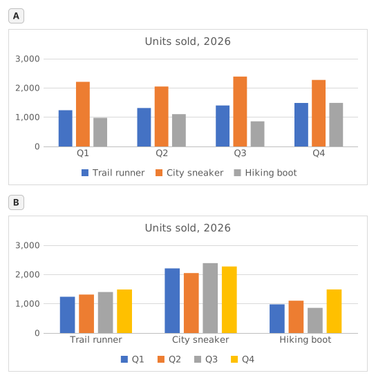
Two clustered column charts titled "Units sold, 2026" drawn from the same table of three models by four quarters: Trail runner Q1 1,240, Q2 1,315, Q3 1,402, Q4 1,488; City sneaker Q1 2,210, Q2 2,050, Q3 2,390, Q4 2,275; Hiking boot Q1 980, Q2 1,105, Q3 860, Q4 1,490. The upper chart, A, has Q1 to Q4 along the horizontal axis and, in each quarter, one column per model; the legend lists Trail runner, City sneaker, Hiking boot. The lower chart, B, has the models along the horizontal axis and, for each model, one column per quarter; the legend lists Q1 to Q4.
  1. Question 1. Chart A was inserted from A1:E4 with Excel's default settings. What did Excel make its data series?

    Answer: The three shoe models

    The data series are the colours listed in the legend, one per model: Trail runner, City sneaker, Hiking boot. Excel chose them because the range has 3 model rows and 4 quarter columns: it puts the larger number of items, the 4 quarters, along the horizontal axis, so each row becomes a series.

  2. Question 2. Chart B shows the same cells A1:E4 as chart A. Which command turns chart A into chart B?

    Answer: Chart Design → Switch Row/Column

    Switch Row/Column (Chart Design tab, Data group) swaps what the chart reads as series and as categories; the cells on the sheet stay exactly as they are. Paste Special → Transpose copies cells and leaves the chart alone, Change Chart Type changes the kind of chart, and Categories in reverse order only flips the order along the axis.

  3. Question 3. The sales director asks: "Did each model sell more in every quarter than in the one before?" Which chart answers that at a glance?

    Answer: Chart B

    Excel draws the series of one category side by side, and neighbouring columns are the easiest to compare. In chart B each model is a category, so its four quarters stand next to each other and a steady rise shows as a staircase (Trail runner); in chart A you would have to follow one colour across four clusters. Same numbers, different comparisons made easy.

  4. Question 4. You insert a clustered column chart from your flipped table G1:J5 (quarters in the rows, models across) with the default settings. What does Excel put along the horizontal axis?

    Answer: The four quarters

    Excel counts the rows and the columns of the range and puts the larger number of items along the horizontal axis: 4 quarters against 3 models, whichever way round the table is. So the flipped table gives the layout of chart A again; for the other layout, use Switch Row/Column on either chart.

Common mistakes

Flipping only the numbers with =TRANSPOSE(B2:E4): the labels are lost and the block lands one row and one column off, so the flipped table and the quarter totals no longer line up with the quarters.

How we grade

Any formula that produces the right result is accepted, unless the task names a function: then another function earns half credit. We compare values with a small tolerance and ignore case and spaces in text. A correct number typed by hand instead of a formula earns half credit. Multi-cell tasks earn full credit at 100% of cells, half credit from 50%. Where it matters, we also change an input cell on a copy of your sheet and check that your formula follows.

Answers computed with Excel 365 rules and checked in our grading engine on November 20, 2026. Author: GridBelt team.

In these programs

  • Excel test in 7 days, Level 1 planDay 6
  • Excel test in 7 days, Level 2 planDay 5
  • Excel for Sales and MarketingDay 7

Related exercises

  • Read a clustered column chart of revenue by regionBeginner, ~6 min
  • Sales by region and product with SUMIFSIntermediate, ~7 min
  • Pick the right chart for each questionBeginner, ~9 min

Function reference

Official documentation

Next exercise

Revenue and margin % in one readable chart