Aller au contenu
GridBelt
  • Test Excel
  • Exercices
  • Programmes
  • Tarifs
Se connecter
Commencer le test gratuit
  • Test Excel
  • Exercices
  • Programmes
  • Tarifs
Se connecterCréer un compte
Commencer le test gratuit
GridBelt

Entraînez-vous sur Excel dans votre navigateur.

Test Excel

  • Niveau 1 : Débutant
  • Niveau 2 : Intermédiaire
  • Niveau 3 : Expert
  • Test Excel en 7 jours
  • Classement
  • Test Excel en entretien d’embauche
  • Évaluation Excel d’Indeed

Exercices

  • Tous les exercices
  • Programmes
  • Pour débutants

Guides

  • Formules Excel
  • Raccourcis Excel

Entreprise

  • À propos
  • Tarifs
  • Comment nous corrigeons

© GridBelt. Tous droits réservés.

  • Politique de confidentialité
  • Conditions d’utilisation
  • Politique de remboursement

Excel est une marque commerciale de Microsoft Corporation. Indeed, TestGorilla, SHL et les autres marques sont la propriété de leurs détenteurs respectifs. GridBelt est un site d’entraînement indépendant ; il n’est affilié ni à Microsoft, ni à TestGorilla, ni à SHL, ni à Indeed, et n’est ni cautionné ni sponsorisé par ces sociétés.

  1. Exercices
  2. /
  3. Charts

Excel combo chart practice: revenue and margin % in one chart

  • Expert
  • ~9 min
  • Charts

Énoncé en anglais

An outdoor-gear shop reviews its 2026 months: revenue, cost of sales and gross profit are in A1:D13. The shop was closed for a refit in February, so that month has no sales at all. The owner wants revenue and gross margin in one chart. The first attempt (chart A) and the second (chart B) are shown below; both plot the margin column E that you are about to fill.

Two charts titled "Revenue and gross margin, 2026", each with revenue as blue columns and gross margin as an orange line with markers, January to December. Revenue: Jan $41,820, Feb $0, Mar $58,430, Apr $66,910, May $74,250, Jun $88,640, Jul $94,370, Aug $91,280, Sep $70,560, Oct $63,190, Nov $72,840, Dec $89,710. Gross margin: Jan 44.1%, Feb #N/A, Mar 35.2%, Apr 33.8%, May 36.7%, Jun 32.9%, Jul 35.8%, Aug 34.1%, Sep 39.6%, Oct 41.2%, Nov 37.4%, Dec 31.8%. In the upper chart, A, both series share one dollar axis on the left from $0 to $100,000, and the margin line runs flat along the bottom. In the lower chart, B, the dollar axis on the left is unchanged and an axis on the right runs from 0% to 50%; the margin line now rises and falls across the tops of the columns. In both charts Feb has no column and no margin point: the line breaks after Jan and starts again at Mar.

Ce que vous devez faire

  1. 1Gross margin is gross profit divided by revenue. Click E2 and divide D2 by B2.
  2. 2February has no revenue, so a plain division shows #DIV/0! there. Wrap it in IFERROR and give NA() as the value to show instead: the cell then shows #N/A, the value a chart leaves out.
  3. 3Fill E2 down to E13 (double-click the fill handle, or Ctrl+D / ⌘D on the selected range), then format E2:E13 as a percentage with one decimal place: Ctrl+Shift+% (Control+Shift+% on a Mac), then Increase Decimal once (in this grid: the toolbar's Increase decimal places button, under ⋮ when the toolbar is narrow; in Excel, Format Cells with Ctrl+1 / ⌘1 → Percentage → 1 decimal place works too). February stays #N/A.
  4. 4Then answer the questions about the two charts. They are pictures: this practice grid has no chart command.

Cellules de réponse

Questions

Choisissez vos réponses ici : le bouton Vérifier les corrige en même temps que les cellules de réponse.

  1. Question 1In chart A, revenue and gross margin share one vertical axis. Why does the margin line lie flat along the bottom?

    Choisissez une réponse.

  2. Question 2Chart B shows the same two series after one change. Which change was it?

    Choisissez une réponse.

  3. Question 3In chart B the margin line has no point for February, because that margin cell holds #N/A. What would the chart show if the formula returned empty text ("") for February instead?

    Choisissez une réponse.

  4. Question 4Which statements about chart B are true? Select all that apply.

    Sélectionnez toutes les réponses correctes.

Correction

Répondez aux questions, saisissez votre formule dans la grille, appuyez sur Enter, puis cliquez sur Vérifier. Nous corrigeons vos réponses, la valeur de chaque cellule de réponse et la formule qui la produit.

Tâches

  1. Non vérifiéIn E2:E13, compute each month's gross margin, gross profit ÷ revenue, with one formula filled down; a month without revenue must return #N/A: wrap the division in IFERROR(…, NA()) (or test the revenue with IF).
  2. Non vérifiéFormat E2:E13 as a percentage with one decimal place (0.0%, for example 35.2%).
  3. Non vérifiéQuestion 1 : In chart A, revenue and gross margin share one vertical axis. Why does the margin line lie flat along the bottom?
  4. Non vérifiéQuestion 2 : Chart B shows the same two series after one change. Which change was it?
  5. Non vérifiéQuestion 3 : In chart B the margin line has no point for February, because that margin cell holds #N/A. What would the chart show if the formula returned empty text ("") for February instead?
  6. Non vérifiéQuestion 4 : Which statements about chart B are true? Select all that apply.

Ordinateur recommandé pour les tâches dans la feuille de calcul. La feuille défile à l’intérieur de ce cadre.

StartInsertFormulasDataView
A1fxPréparation de votre classeur…
A
B
C
D
E
F
G
H
I
J
1
2
3
4
5
6
7
8
9
10
11
12
13
14
15
16
17
18
19
20
21
22
Sheet1

Répondez aux questions, remplissez les cellules, puis vérifiez.

À propos de cet exercice

Un jeu de données de 12 lignes sur une feuille, une cellule de réponse, environ 9 minutes. Corrigé dans votre navigateur : la valeur et la formule qui la produit, avec des indications sur la correction à apporter. L’exercice pose aussi 4 questions à choix multiple, corrigées par le même bouton Vérifier.

Comment le résoudre

  • E2=IFERROR(D2/B2,NA())

=IFERROR(D2/B2,NA()) divides gross profit by revenue and, for February's 0 ÷ 0, returns #N/A instead of #DIV/0!; formatted as 0.0% the margins read 44.1%, 35.2% and so on. In chart A the margins (all below 0.5) share a dollar axis built for tens of thousands, so the line looks flat; chart B moves the margin to a secondary axis with its own scale from 0% to 50%. #N/A keeps February out of the line, whereas "" would be plotted as 0%. In chart B you read the margin on the right-hand axis, the crossings of line and columns mean nothing, and the best margin (January) is not the best gross profit (July).

For an existing chart, two routes in Excel 365: right-click the margin line → Format Data Series → Series Options → Secondary Axis (Windows and Mac); or select the chart → Chart Design → Change Chart Type → Combo, set Gross margin to Line and tick its Secondary Axis box (Windows). Insert → Insert Combo Chart → Clustered Column – Line on Secondary Axis builds such a chart from scratch: select A1:B13, add E1:E13 with Ctrl (⌘ on a Mac), and the margin, the second series, becomes the line. Excel 2016–2019 for Windows work the same way; the tab is called Design, under Chart Tools. Use a secondary axis for a second unit, percent next to dollars; two dollar series belong on one axis, or readers compare heights measured against different scales. Add axis titles (Chart Design → Add Chart Element → Axis Titles) so nobody reads the margin against dollars. Charts plot "" as zero, so chart data should return NA(). #N/A never becomes a point. With Select Data → Hidden and Empty Cells → Show #N/A as an empty cell ticked (new charts in Excel 365 have it on) and empty cells shown as Gaps, the line breaks at February, as in chart B; with that box cleared, it runs straight from January to March. For a table people read, a text such as n/a is friendlier (see the IFERROR margin exercise). IFERROR also hides other errors, such as a text value in a revenue cell; =IF(B2=0,NA(),D2/B2) guards only the zero.

Autres méthodes valables

  • =IF(B2=0,NA(),D2/B2) — guards only the zero revenue and lets any other error show
  • =IFERROR((B2-C2)/B2,NA()) — the margin straight from revenue and cost of sales
  • =IF(ISERROR(D2/B2),NA(),D2/B2) — the pre-2007 pattern, same result

Réponses aux questions
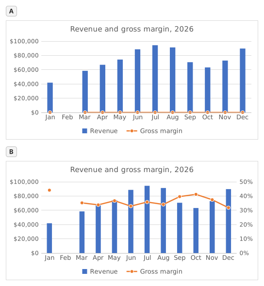
Two charts titled "Revenue and gross margin, 2026", each with revenue as blue columns and gross margin as an orange line with markers, January to December. Revenue: Jan $41,820, Feb $0, Mar $58,430, Apr $66,910, May $74,250, Jun $88,640, Jul $94,370, Aug $91,280, Sep $70,560, Oct $63,190, Nov $72,840, Dec $89,710. Gross margin: Jan 44.1%, Feb #N/A, Mar 35.2%, Apr 33.8%, May 36.7%, Jun 32.9%, Jul 35.8%, Aug 34.1%, Sep 39.6%, Oct 41.2%, Nov 37.4%, Dec 31.8%. In the upper chart, A, both series share one dollar axis on the left from $0 to $100,000, and the margin line runs flat along the bottom. In the lower chart, B, the dollar axis on the left is unchanged and an axis on the right runs from 0% to 50%; the margin line now rises and falls across the tops of the columns. In both charts Feb has no column and no margin point: the line breaks after Jan and starts again at Mar.
  1. Question 1. In chart A, revenue and gross margin share one vertical axis. Why does the margin line lie flat along the bottom?

    Réponse : Margins below 0.5 share an axis built for dollars

    On one axis every series uses the same scale: the axis runs to $100,000 for the revenue, so margins between 31.8% and 44.1% (0.32 to 0.44 as numbers) sit a hair above zero and every change disappears. The margin did move; it only needs its own scale.

  2. Question 2. Chart B shows the same two series after one change. Which change was it?

    Réponse : Gross margin series → Format Data Series → Secondary Axis

    Putting the margin on a secondary axis gives it its own scale on the right (0% to 50% here) while revenue keeps the dollar axis on the left. A Maximum of 1 would cut every revenue column off at the top, Display units only relabels the axis in thousands without changing the scale, and Switch Row/Column would turn the months into series.

  3. Question 3. In chart B the margin line has no point for February, because that margin cell holds #N/A. What would the chart show if the formula returned empty text ("") for February instead?

    Réponse : A point at 0% for February

    A formula that returns "" leaves text in the cell, not an empty cell, and Excel plots text in a line or column series as 0, so the line would dive to 0% in February. #N/A is never plotted as a point: chart B shows it as an empty cell, a gap (Select Data → Hidden and Empty Cells → Show #N/A as an empty cell), and with that box cleared the line would run straight from January to March, still without a February point.

  4. Question 4. Which statements about chart B are true? Select all that apply.

    Réponses : You read the margin on the right-hand axis et Where the line crosses a column means nothing

    The margin is plotted against the right-hand axis and the revenue against the left-hand one, so a point where the line meets a column only reflects how the two scales happen to be set. The highest margin, January's 44.1%, comes from a quiet month: July's 35.8% on far more revenue earned more gross profit ($33,780 against $18,440).

Erreurs fréquentes

Using =IFERROR(D2/B2,"") or =IFERROR(D2/B2,0): the table looks tidy, but a chart draws February at 0% and the margin line dives to the bottom; NA() keeps the month out of the chart.

Comment nous corrigeons

Toute formule qui produit le bon résultat est acceptée, sauf si la tâche nomme une fonction : une autre fonction rapporte alors la moitié des points. Nous comparons les valeurs avec une petite tolérance et ignorons la casse et les espaces dans le texte. Un nombre correct saisi à la main au lieu d’une formule rapporte la moitié des points. Les tâches sur plusieurs cellules rapportent tous les points avec 100 % de cellules justes, la moitié à partir de 50 %. Lorsque c’est pertinent, nous modifions aussi une cellule d’entrée sur une copie de votre feuille et vérifions que votre formule suit.

Réponses calculées selon les règles d’Excel 365 et vérifiées dans notre correcteur le 20 novembre 2026. Auteur : GridBelt team.

Dans ces programmes

  • Excel test in 7 days, Plan de niveau 3Jour 6
  • Excel for Data AnalystsJour 11
  • Excel for Accounting and BookkeepingJour 9

Exercices associés

  • Margin % without #DIV/0!Intermédiaire, ~6 min
  • Spot a misleading chart axis and measure the real differenceIntermédiaire, ~8 min
  • Share of total per region, formatted as %Débutant, ~5 min

Référence de la fonction

Documentation officielle