Aller au contenu
GridBelt
  • Test Excel
  • Exercices
  • Programmes
  • Tarifs
Se connecter
Commencer le test gratuit
  • Test Excel
  • Exercices
  • Programmes
  • Tarifs
Se connecterCréer un compte
Commencer le test gratuit
GridBelt

Entraînez-vous sur Excel dans votre navigateur.

Test Excel

  • Niveau 1 : Débutant
  • Niveau 2 : Intermédiaire
  • Niveau 3 : Expert
  • Test Excel en 7 jours
  • Classement
  • Test Excel en entretien d’embauche
  • Évaluation Excel d’Indeed

Exercices

  • Tous les exercices
  • Programmes
  • Pour débutants

Guides

  • Formules Excel
  • Raccourcis Excel

Entreprise

  • À propos
  • Tarifs
  • Comment nous corrigeons

© GridBelt. Tous droits réservés.

  • Politique de confidentialité
  • Conditions d’utilisation
  • Politique de remboursement

Excel est une marque commerciale de Microsoft Corporation. Indeed, TestGorilla, SHL et les autres marques sont la propriété de leurs détenteurs respectifs. GridBelt est un site d’entraînement indépendant ; il n’est affilié ni à Microsoft, ni à TestGorilla, ni à SHL, ni à Indeed, et n’est ni cautionné ni sponsorisé par ces sociétés.

  1. Exercices
  2. /
  3. Charts

Excel chart practice: spot a misleading axis that does not start at zero

  • Intermédiaire
  • ~8 min
  • Charts

Énoncé en anglais

A home-improvement chain surveys its customers every month. The regional manager's slide shows the 2026 satisfaction scores (0 to 100) of five stores as columns on a vertical axis that starts at 95, and one store looks far ahead of the rest; the manager wants to reward it. Before the meeting, measure the real difference in the sheet: the scores are in A1:B6 and the slide's axis minimum is in F2.

Two column charts titled "Customer satisfaction score, 2026" with the same five store scores, each column labelled: Harbor 98.6, Riverside 97.8, Station 95.9, Old Town 97.1, Airport 96.5. Chart A, as on the slide, has a vertical axis from 95 to 99, so each column shows only the part of the score above 95: Harbor's column towers over Station's. Chart B has a vertical axis from 0 to 100, and the five columns look almost the same height.

Ce que vous devez faire

  1. 1Click C2 and compare the store with the lowest score of all five: divide B2 by MIN($B$2:$B$6) and subtract 1. The $ signs keep MIN on all five stores when you fill down — F4 (Windows) or ⌘T (Mac) adds them.
  2. 2Fill C2 down to C6, then format C2:C6 as a percentage with one decimal place: Ctrl+Shift+% (Control+Shift+% on a Mac), then Increase Decimal once (in this grid: the toolbar's Increase decimal places button, under ⋮ when the toolbar is narrow; in Excel, Format Cells with Ctrl+1 / ⌘1 → Percentage → 1 decimal place works too). The lowest store shows 0.0%.
  3. 3On a chart, a column is drawn from the axis minimum up to its value, so its drawn height is the value minus the minimum. In F3, divide the drawn height of the tallest column by that of the shortest: (MAX(B2:B6) − F2) ÷ (MIN(B2:B6) − F2). Refer to F2 and do not type the minimum into the formula, so that F3 still works when the axis minimum changes.
  4. 4Then answer the questions; the charts are pictures, because this practice grid has no chart command.

Cellules de réponse

Questions

Choisissez vos réponses ici : le bouton Vérifier les corrige en même temps que les cellules de réponse.

  1. Question 1On the slide (chart A), Harbor's column towers over Station's. How much higher is Harbor's score really? Use your column C.

    Choisissez une réponse.

  2. Question 2You select the slide's vertical axis and open Format Axis (right-click the axis → Format Axis). Which change makes the columns honest?

    Choisissez une réponse.

    The slide's column chart "Customer satisfaction score, 2026", narrower here, with the store names slanted; its vertical axis (95 to 99) is selected, and the Format Axis pane is open at Axis Options. Under Bounds, Minimum shows 95.0 with a Reset button next to it and Maximum shows 99.0 with an Auto button; under Units, Major shows 1.0 and Minor 0.2, both Auto.
  3. Question 3In which of these charts is a value axis that does not start at 0 acceptable? Select all that apply.

    Sélectionnez toutes les réponses correctes.

Correction

Répondez aux questions, saisissez votre formule dans la grille, appuyez sur Enter, puis cliquez sur Vérifier. Nous corrigeons vos réponses, la valeur de chaque cellule de réponse et la formule qui la produit.

Tâches

  1. Non vérifiéIn C2:C6, compute how much higher each store's score is than the lowest of the five scores, as a share of the lowest — score ÷ lowest − 1 — with one formula filled down.
  2. Non vérifiéFormat C2:C6 as a percentage with one decimal place (0.0%, for example 1.2%).
  3. Non vérifiéIn F3, compute how many times taller the tallest column is drawn than the shortest on an axis that starts at the value in F2: (highest score − F2) ÷ (lowest score − F2).
  4. Non vérifiéQuestion 1 : On the slide (chart A), Harbor's column towers over Station's. How much higher is Harbor's score really? Use your column C.
  5. Non vérifiéQuestion 2 : You select the slide's vertical axis and open Format Axis (right-click the axis → Format Axis). Which change makes the columns honest?
  6. Non vérifiéQuestion 3 : In which of these charts is a value axis that does not start at 0 acceptable? Select all that apply.

Ordinateur recommandé pour les tâches dans la feuille de calcul. La feuille défile à l’intérieur de ce cadre.

StartInsertFormulasDataView
A1fxPréparation de votre classeur…
A
B
C
D
E
F
G
H
I
J
1
2
3
4
5
6
7
8
9
10
11
12
13
14
15
16
17
18
19
20
21
22
Sheet1

Répondez aux questions, remplissez les cellules, puis vérifiez.

À propos de cet exercice

Un jeu de données de 5 lignes sur une feuille, 2 cellules de réponse, environ 8 minutes. Corrigé dans votre navigateur : la valeur et la formule qui la produit, avec des indications sur la correction à apporter. L’exercice pose aussi 3 questions à choix multiple, corrigées par le même bouton Vérifier.

Comment le résoudre

  • C2=B2/MIN($B$2:$B$6)-1
  • F3=(MAX(B2:B6)-F2)/(MIN(B2:B6)-F2)

Harbor's score is only 2.8% above Station's (=B2/MIN($B$2:$B$6)-1), but on an axis that starts at 95 a column only shows the part of its value above 95, so Harbor's 3.6 points against Station's 0.9 draw a column 4.0 times as tall (F3). With the axis from 0 the drawn heights are the real values and the ratio falls to 1.03. The fix is to type 0 as the axis Minimum; a non-zero axis is acceptable for lines and dots, which show values by position rather than by length.

In Excel, right-click the vertical axis → Format Axis → Axis Options → Bounds and type 0 in Minimum (the same pane on Windows and Mac, and in Excel 2016–2021). When a bound is on Auto, Excel chooses it: if the smallest value is above about five sixths of the largest, the automatic minimum is not 0, so five scores between 95.9 and 98.6 get a cut axis even if nobody set one, and Reset only returns to that automatic value. The picture shows a 300% difference where the data has 2.8%; Tufte called the ratio of the two the lie factor. When small differences matter, chart them directly: columns of each store's gap to the lowest store or to a target, a dot plot, or a line with a clearly labelled axis. Pitfall: =B2/MIN(B2:B6)-1 without $ slides the MIN range down as you fill, so the stores below Station are compared with a different "lowest" score.

Autres méthodes valables

  • =B2/MIN(B$2:B$6)-1 — locking the rows is enough when you only fill down
  • =(B2-MIN($B$2:$B$6))/MIN($B$2:$B$6) — the same, written as (score − lowest) ÷ lowest
  • =(MAX(B2:B6)-$F$2)/(MIN(B2:B6)-$F$2) in F3 — the same with F2 locked

Réponses aux questions
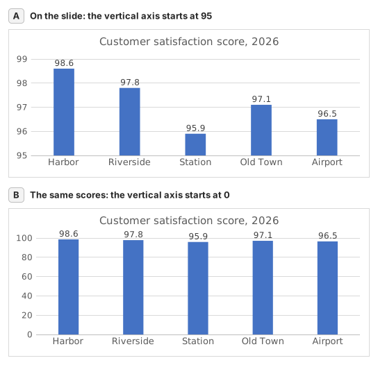
Two column charts titled "Customer satisfaction score, 2026" with the same five store scores, each column labelled: Harbor 98.6, Riverside 97.8, Station 95.9, Old Town 97.1, Airport 96.5. Chart A, as on the slide, has a vertical axis from 95 to 99, so each column shows only the part of the score above 95: Harbor's column towers over Station's. Chart B has a vertical axis from 0 to 100, and the five columns look almost the same height.
  1. Question 1. On the slide (chart A), Harbor's column towers over Station's. How much higher is Harbor's score really? Use your column C.

    Réponse : About 3% higher

    Harbor scores 98.6 and Station 95.9, so Harbor is 98.6 ÷ 95.9 − 1 ≈ 2.8% higher. On the slide each column only shows the part above 95: 3.6 points against 0.9, which draws Harbor's column 4.0 times as tall.

  2. Question 2. You select the slide's vertical axis and open Format Axis (right-click the axis → Format Axis). Which change makes the columns honest?

    Réponse : Type 0 in the Minimum box

    Columns show a value by their length from the axis, so the axis must start at 0 for the lengths to compare. Reset is not enough: when every value is above about five sixths of the largest one, as here, Excel's automatic minimum is not 0 either. Data labels print the true numbers but leave the misleading lengths.

  3. Question 3. In which of these charts is a value axis that does not start at 0 acceptable? Select all that apply.

    Réponses : A line chart of a share price moving between $95 and $99 et A scatter chart of house size against sale price

    Columns and bars show a value by their length, so a cut axis turns small gaps into big ones. Lines and dots show a value by its position, so their axis may zoom into the range where the values move, as long as its labels show where it starts.

Erreurs fréquentes

Filling =B2/MIN(B2:B6)-1 down without $: in the rows below Station the MIN range no longer includes Station's score, so those stores are measured against the wrong lowest store.

Comment nous corrigeons

Toute formule qui produit le bon résultat est acceptée, sauf si la tâche nomme une fonction : une autre fonction rapporte alors la moitié des points. Nous comparons les valeurs avec une petite tolérance et ignorons la casse et les espaces dans le texte. Un nombre correct saisi à la main au lieu d’une formule rapporte la moitié des points. Les tâches sur plusieurs cellules rapportent tous les points avec 100 % de cellules justes, la moitié à partir de 50 %. Lorsque c’est pertinent, nous modifions aussi une cellule d’entrée sur une copie de votre feuille et vérifions que votre formule suit.

Réponses calculées selon les règles d’Excel 365 et vérifiées dans notre correcteur le 20 novembre 2026. Auteur : GridBelt team.

Exercices associés

  • Read a clustered column chart of revenue by regionDébutant, ~6 min
  • Year-over-year % changeDébutant, ~4 min
  • Revenue and margin % in one readable chartExpert, ~9 min

Référence de la fonction

Documentation officielle

Exercice suivant

Series or categories? Read a chart both ways and flip its table