Aller au contenu
GridBelt
  • Test Excel
  • Exercices
  • Programmes
  • Tarifs
Se connecter
Commencer le test gratuit
  • Test Excel
  • Exercices
  • Programmes
  • Tarifs
Se connecterCréer un compte
Commencer le test gratuit
GridBelt

Entraînez-vous sur Excel dans votre navigateur.

Test Excel

  • Niveau 1 : Débutant
  • Niveau 2 : Intermédiaire
  • Niveau 3 : Expert
  • Test Excel en 7 jours
  • Classement
  • Test Excel en entretien d’embauche
  • Évaluation Excel d’Indeed

Exercices

  • Tous les exercices
  • Programmes
  • Pour débutants

Guides

  • Formules Excel
  • Raccourcis Excel

Entreprise

  • À propos
  • Tarifs
  • Comment nous corrigeons

© GridBelt. Tous droits réservés.

  • Politique de confidentialité
  • Conditions d’utilisation
  • Politique de remboursement

Excel est une marque commerciale de Microsoft Corporation. Indeed, TestGorilla, SHL et les autres marques sont la propriété de leurs détenteurs respectifs. GridBelt est un site d’entraînement indépendant ; il n’est affilié ni à Microsoft, ni à TestGorilla, ni à SHL, ni à Indeed, et n’est ni cautionné ni sponsorisé par ces sociétés.

  1. Exercices
  2. /
  3. Charts

Excel chart practice: series, categories and a flipped table

  • Intermédiaire
  • ~7 min
  • Charts

Énoncé en anglais

An outdoor-footwear brand tracks the 2026 unit sales of three of its shoe models in A1:E4, quarter by quarter: models down the rows, quarters across. The analyst's two clustered column charts of that range are shown below. The planning sheet also needs the same numbers the other way round, quarters down the rows, as a live formula, with a total for each quarter.

Two clustered column charts titled "Units sold, 2026" drawn from the same table of three models by four quarters: Trail runner Q1 1,240, Q2 1,315, Q3 1,402, Q4 1,488; City sneaker Q1 2,210, Q2 2,050, Q3 2,390, Q4 2,275; Hiking boot Q1 980, Q2 1,105, Q3 860, Q4 1,490. The upper chart, A, has Q1 to Q4 along the horizontal axis and, in each quarter, one column per model; the legend lists Trail runner, City sneaker, Hiking boot. The lower chart, B, has the models along the horizontal axis and, for each model, one column per quarter; the legend lists Q1 to Q4.

Ce que vous devez faire

  1. 1Click G1, type =TRANSPOSE(A1:E4) and press Enter. The result spills into G1:J5: the corner label and the quarters run down column G, the models across row 1. Keep G1:J5 empty, or the formula shows #SPILL!. (Excel 2019 and older: select G1:J5 first, type the formula and confirm it as an array formula with Ctrl+Shift+Enter on Windows or ⌘+Shift+Return on a Mac.)
  2. 2The flipped copy is linked to A1:E4: when a number there changes, G1:J5 changes with it, unlike a copy made with Paste Special → Transpose.
  3. 3In K2, add up the quarter in row 2 of the flipped table: a SUM over H2:J2, its three model cells. Fill K2 down to K5 (double-click the fill handle, or select K2:K5 and press Ctrl+D / ⌘D).
  4. 4Then answer the questions about the two charts. They are pictures: this practice grid has no chart command.

Cellules de réponse

Questions

Choisissez vos réponses ici : le bouton Vérifier les corrige en même temps que les cellules de réponse.

  1. Question 1Chart A was inserted from A1:E4 with Excel's default settings. What did Excel make its data series?

    Choisissez une réponse.

  2. Question 2Chart B shows the same cells A1:E4 as chart A. Which command turns chart A into chart B?

    Choisissez une réponse.

  3. Question 3The sales director asks: "Did each model sell more in every quarter than in the one before?" Which chart answers that at a glance?

    Choisissez une réponse.

  4. Question 4You insert a clustered column chart from your flipped table G1:J5 (quarters in the rows, models across) with the default settings. What does Excel put along the horizontal axis?

    Choisissez une réponse.

Correction

Répondez aux questions, saisissez votre formule dans la grille, appuyez sur Enter, puis cliquez sur Vérifier. Nous corrigeons vos réponses, la valeur de chaque cellule de réponse et la formule qui la produit.

Tâches

  1. Non vérifiéIn G1, flip the table A1:E4 with one TRANSPOSE formula, labels included, so the quarters run down the rows and the models across (the result spills into G1:J5).
  2. Non vérifiéIn K2:K5, total each quarter's units across the three models of your flipped table, with one formula filled down.
  3. Non vérifiéQuestion 1 : Chart A was inserted from A1:E4 with Excel's default settings. What did Excel make its data series?
  4. Non vérifiéQuestion 2 : Chart B shows the same cells A1:E4 as chart A. Which command turns chart A into chart B?
  5. Non vérifiéQuestion 3 : The sales director asks: "Did each model sell more in every quarter than in the one before?" Which chart answers that at a glance?
  6. Non vérifiéQuestion 4 : You insert a clustered column chart from your flipped table G1:J5 (quarters in the rows, models across) with the default settings. What does Excel put along the horizontal axis?

Ordinateur recommandé pour les tâches dans la feuille de calcul. La feuille défile à l’intérieur de ce cadre.

StartInsertFormulasDataView
A1fxPréparation de votre classeur…
A
B
C
D
E
F
G
H
I
J
1
2
3
4
5
6
7
8
9
10
11
12
13
14
15
16
17
18
19
20
21
22
Sheet1

Répondez aux questions, remplissez les cellules, puis vérifiez.

À propos de cet exercice

Un jeu de données de 3 lignes sur une feuille, 2 cellules de réponse, environ 7 minutes. Corrigé dans votre navigateur : la valeur et la formule qui la produit, avec des indications sur la correction à apporter. L’exercice pose aussi 4 questions à choix multiple, corrigées par le même bouton Vérifier.

Comment le résoudre

  • G1=TRANSPOSE(A1:E4)
  • K2=SUM(H2:J2)

TRANSPOSE returns the table with its rows and columns swapped: =TRANSPOSE(A1:E4) puts the quarters down column G and the models across row 1, and because it is a formula the copy follows every change in A1:E4. Each quarter then sits in one row, so its total is a plain SUM across that row. The charts: Excel made the models the series of chart A because the range has fewer models than quarters; Chart Design → Switch Row/Column turns it into chart B without touching the cells; chart B puts each model's four quarters side by side, which answers "did it grow every quarter?"; and a chart of the flipped table again gets the quarters along the axis, because Excel puts the larger number of items there.

Where it lives: select the chart, then Chart Design → Data group → Switch Row/Column (in Excel 2016–2019 the tab is called Design, under Chart Tools); Chart Design → Select Data opens the same switch together with the series and category ranges, which is where you fix a chart whose series are wrong. Excel's rule (Microsoft Support): it compares the rows and columns of the selected range and puts the larger number along the horizontal axis; with as many rows as columns, each row becomes a series. Pitfall 1: Paste Special → Transpose makes a static copy that does not follow later changes, while TRANSPOSE stays linked. Pitfall 2: an empty corner cell comes out as 0 in Excel's TRANSPOSE result; a label such as Units in A1 avoids that. Pitfall 3: in Excel 2019 and older, TRANSPOSE is a legacy array formula over a selected block (Ctrl+Shift+Enter) that you can only edit or delete as a whole; in Excel 365 it spills from one cell.

Autres méthodes valables

  • =TRANSPOSE($A$1:$E$4) in G1 — the same; the $ signs make no difference to a single formula
  • =H2+I2+J2 in K2 — the same total as =SUM(H2:J2), filled down
  • =SUM(B2:B4) in K2, =SUM(C2:C4) in K3 and so on — the totals straight from the original table, one formula per quarter (it cannot be filled down)

Réponses aux questions
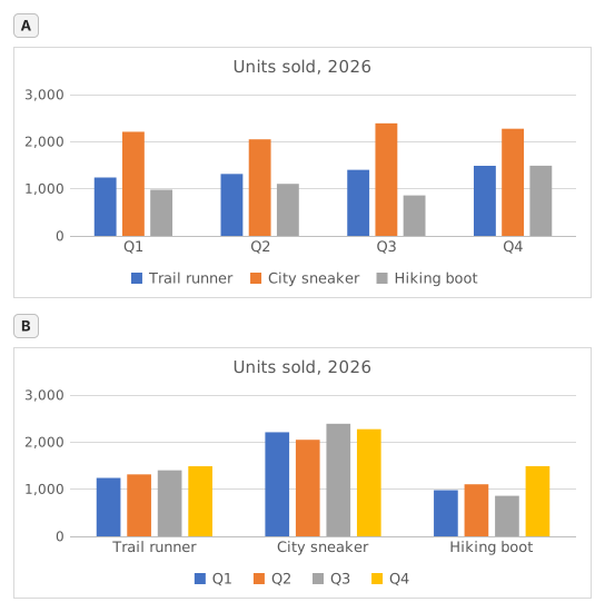
Two clustered column charts titled "Units sold, 2026" drawn from the same table of three models by four quarters: Trail runner Q1 1,240, Q2 1,315, Q3 1,402, Q4 1,488; City sneaker Q1 2,210, Q2 2,050, Q3 2,390, Q4 2,275; Hiking boot Q1 980, Q2 1,105, Q3 860, Q4 1,490. The upper chart, A, has Q1 to Q4 along the horizontal axis and, in each quarter, one column per model; the legend lists Trail runner, City sneaker, Hiking boot. The lower chart, B, has the models along the horizontal axis and, for each model, one column per quarter; the legend lists Q1 to Q4.
  1. Question 1. Chart A was inserted from A1:E4 with Excel's default settings. What did Excel make its data series?

    Réponse : The three shoe models

    The data series are the colours listed in the legend, one per model: Trail runner, City sneaker, Hiking boot. Excel chose them because the range has 3 model rows and 4 quarter columns: it puts the larger number of items, the 4 quarters, along the horizontal axis, so each row becomes a series.

  2. Question 2. Chart B shows the same cells A1:E4 as chart A. Which command turns chart A into chart B?

    Réponse : Chart Design → Switch Row/Column

    Switch Row/Column (Chart Design tab, Data group) swaps what the chart reads as series and as categories; the cells on the sheet stay exactly as they are. Paste Special → Transpose copies cells and leaves the chart alone, Change Chart Type changes the kind of chart, and Categories in reverse order only flips the order along the axis.

  3. Question 3. The sales director asks: "Did each model sell more in every quarter than in the one before?" Which chart answers that at a glance?

    Réponse : Chart B

    Excel draws the series of one category side by side, and neighbouring columns are the easiest to compare. In chart B each model is a category, so its four quarters stand next to each other and a steady rise shows as a staircase (Trail runner); in chart A you would have to follow one colour across four clusters. Same numbers, different comparisons made easy.

  4. Question 4. You insert a clustered column chart from your flipped table G1:J5 (quarters in the rows, models across) with the default settings. What does Excel put along the horizontal axis?

    Réponse : The four quarters

    Excel counts the rows and the columns of the range and puts the larger number of items along the horizontal axis: 4 quarters against 3 models, whichever way round the table is. So the flipped table gives the layout of chart A again; for the other layout, use Switch Row/Column on either chart.

Erreurs fréquentes

Flipping only the numbers with =TRANSPOSE(B2:E4): the labels are lost and the block lands one row and one column off, so the flipped table and the quarter totals no longer line up with the quarters.

Comment nous corrigeons

Toute formule qui produit le bon résultat est acceptée, sauf si la tâche nomme une fonction : une autre fonction rapporte alors la moitié des points. Nous comparons les valeurs avec une petite tolérance et ignorons la casse et les espaces dans le texte. Un nombre correct saisi à la main au lieu d’une formule rapporte la moitié des points. Les tâches sur plusieurs cellules rapportent tous les points avec 100 % de cellules justes, la moitié à partir de 50 %. Lorsque c’est pertinent, nous modifions aussi une cellule d’entrée sur une copie de votre feuille et vérifions que votre formule suit.

Réponses calculées selon les règles d’Excel 365 et vérifiées dans notre correcteur le 20 novembre 2026. Auteur : GridBelt team.

Dans ces programmes

  • Excel test in 7 days, Plan de niveau 1Jour 6
  • Excel test in 7 days, Plan de niveau 2Jour 5
  • Excel for Sales and MarketingJour 7

Exercices associés

  • Read a clustered column chart of revenue by regionDébutant, ~6 min
  • Sales by region and product with SUMIFSIntermédiaire, ~7 min
  • Pick the right chart for each questionDébutant, ~9 min

Référence de la fonction

Documentation officielle

Exercice suivant

Revenue and margin % in one readable chart