À propos de cet exercice
Un jeu de données de 7 lignes sur une feuille, une cellule de réponse, environ 6 minutes. Corrigé dans votre navigateur : la valeur et la formule qui la produit, avec des indications sur la correction à apporter. L’exercice pose aussi 4 questions à choix multiple, corrigées par le même bouton Vérifier.
Comment le résoudre
- D2
=(C2-B2)/B2
Growth is the change divided by the starting value: =(C2-B2)/B2 gives the first region's 2026 change as a share of 2025, and filling down to the Total row gives the company's rate to compare with; the 0.0% format shows 0.044 as 4.4%. Reading the chart: the legend says orange is 2026; the biggest dollar increase is the widest gap between a region's two columns (Southeast); the only orange column shorter than its blue partner is Midwest's; and column D shows that Southeast, Southwest and Mountain grew faster than the company.
In Excel: select A1:C7 (leave the Total row out, or its two columns dwarf every region) and choose Insert → Insert Column or Bar Chart → Clustered Column; Excel makes the two year columns the series because the range has more rows than columns. Data labels: Chart Design → Add Chart Element → Data Labels (the tab is called Design, under Chart Tools, in Excel 2016–2019); the number format code #,##0, (Format Axis or Format Data Labels → Number) shows thousands, 879,400 as 879. Pitfall 1: a chart compares heights, so it shows dollar differences; growth in percent needs the calculation, and a small region can grow fastest with the shortest columns. Pitfall 2: if the year headers were numbers instead of text, Excel could plot them as data; clearing the corner cell A1 or storing the years as text keeps them as series names (fix an existing chart with Chart Design → Select Data). Pitfall 3: =C2-B2/B2 without brackets divides first and returns a huge number instead of a percentage.
Autres méthodes valables
- =C2/B2-1 — the same result, shorter
- =(C2-B2)/ABS(B2) — also right when a starting value can be negative (not the case for revenue)
- =IFERROR((C2-B2)/B2,"") — blank instead of #DIV/0! for a region that is new this year
Réponses aux questions
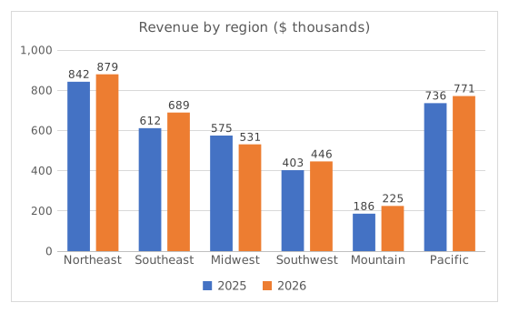
Question 1. In the chart, what do the orange columns show?
Réponse : Revenue in 2026
The legend under the chart maps each colour to a series: blue is 2025 and orange is 2026. A clustered column chart draws one column per series in every category, side by side, so each region gets a 2025 column and a 2026 column.
Question 2. Judging by the chart, which region added the most revenue in dollars from 2025 to 2026?
Réponse : Southeast region
Compare the gap between each region's two columns, not the height of the orange one: Southeast goes from about 612 to 689 thousand, about $78K more, the widest gap. Northeast has the tallest columns but adds only about $37K.
Question 3. Which region's revenue fell from 2025 to 2026?
Réponse : Midwest region
Midwest is the only region whose orange 2026 column is shorter than its blue 2025 column (about 575 down to 531 thousand). Mountain has the shortest columns, but small is not the same as falling: its 2026 column is the taller of its pair.
Question 4. Now look at your column D. Which regions grew faster in percent than the company as a whole (the Total row)? Select all that apply.
Réponses : Southeast region, Southwest region et Mountain region
The company grew by 5.6%. Southeast (12.7%), Southwest (10.8%) and Mountain (20.6%) beat that. Mountain has the highest rate of all although its columns are the shortest: a percentage divides the increase by the starting value, and a small start makes a modest gain a big percentage.
Erreurs fréquentes
Typing =C2-B2/B2 without brackets: Excel divides B2 by itself first and returns the 2026 revenue minus 1 (879,399 for Northeast) instead of a growth rate. Wrap the difference in brackets: =(C2-B2)/B2.
Comment nous corrigeons
Toute formule qui produit le bon résultat est acceptée, sauf si la tâche nomme une fonction : une autre fonction rapporte alors la moitié des points. Nous comparons les valeurs avec une petite tolérance et ignorons la casse et les espaces dans le texte. Un nombre correct saisi à la main au lieu d’une formule rapporte la moitié des points. Les tâches sur plusieurs cellules rapportent tous les points avec 100 % de cellules justes, la moitié à partir de 50 %. Lorsque c’est pertinent, nous modifions aussi une cellule d’entrée sur une copie de votre feuille et vérifions que votre formule suit.
Réponses calculées selon les règles d’Excel 365 et vérifiées dans notre correcteur le 20 novembre 2026. Auteur : GridBelt team.