À propos de cet exercice
Un jeu de données de 150 lignes sur une feuille, 3 cellules de réponse, environ 12 minutes. Corrigé dans votre navigateur : la valeur et la formule qui la produit, avec des indications sur la correction à apporter. L’exercice pose aussi 4 questions à choix multiple, corrigées par le même bouton Vérifier.
Comment le résoudre
- G2
=IF(F2="",0,VALUE(F2)) - J2
=SUMPRODUCT(--ISTEXT(F2:F151)) - J3
=SUM(G2:G151)
Excel sums a value field only when every cell of it is a number. Here some amounts are text (they sit at the left of the cell) and some are blank, so the PivotTable fell back to Count of Amount, which counts every non-empty cell like COUNTA. Picking Sum without cleaning adds the text amounts as 0, so the totals come out too low: convert them first (column G), then summarize by Sum. Department belongs in Rows for one row per department, and rows pasted below a fixed source range stay outside it until you change the data source, or use an Excel Table, which grows with the data.
In desktop Excel you can fix column F in place instead of using a helper column: select F2:F151 and use the warning button next to the green triangles → Convert to Number, or Data → Text to Columns → Finish, or copy a cell that holds 1 and use Paste Special → Multiply. VALUE reads text with your own regional settings; if your Excel uses a comma as the decimal separator, =NUMBERVALUE(F2,".") reads these dot-decimal amounts correctly. Blanks: fill them with 0 (Home → Find & Select → Go To Special → Blanks, type 0, Ctrl+Enter) or keep them and pick Sum yourself. A formula that returns "" for an empty amount returns text, which keeps the field on Count. Then refresh (PivotTable Analyze → Refresh, Alt+F5 on Windows; the tab is called Analyze in Excel 2016 and 2019) and set the field to Sum: right-click a value → Summarize Values By → Sum, or Value Field Settings. Change Data Source sits on the same tab; an Excel Table (Insert → Table) grows with every row added below it, so the PivotTable picks new rows up at the next Refresh. Auto Refresh, which Microsoft lists as a Microsoft 365 Insider feature for now, refreshes PivotTables on workbook data by itself, but it never stretches a fixed range either. This in-browser grid has no PivotTable: the pictures show what Excel does, and your formulas are graded in the grid.
Autres méthodes valables
- =F2*1 or =--F2 in G2 — arithmetic turns text into a number and an empty cell into 0
- =COUNTIF(F2:F151,"*") or =COUNTA(F2:F151)-COUNT(F2:F151) in J2 — other ways to count the text cells
- =SUMPRODUCT(--F2:F151) in J3 — the clean total in one formula, without column G
Réponses aux questions
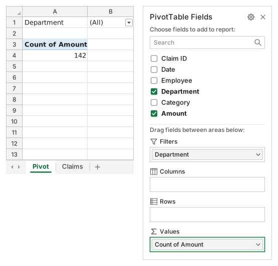
Question 1. Which of these make Excel summarize Amount as Count instead of Sum when the field is dropped into Values? Select all that apply.
Réponses : Some amounts are stored as text et Some amount cells are blank
Excel sums a value field only when every cell of it holds a number; text that looks like a number or an empty cell makes it fall back to Count, which counts non-empty cells like COUNTA (142 of the 150 claims here). Where Department sits, decimals and refreshing play no part in that choice.
Question 2. Suppose you change nothing in the data and only pick Sum in Value Field Settings, as pictured. What will Sum of Amount show?
Réponse : Too little: the text amounts are added as 0
A PivotTable adds only real numbers: blank or nonnumeric values become 0 when the field is summed. The text amounts drop out of every total without any warning, so convert them first (your column G) and then summarize by Sum.
Question 3. A week later, 12 new claims are pasted below the list, in rows 152 to 163 (pictured). After Refresh the report still leaves them out. Which of these make the report include them? Select all that apply.
Réponses : Change Data Source so the range ends at row 163 et Make the claims an Excel Table and use it as the source
The PivotTable reads the fixed range Claims!$A$1:$F$151, and Refresh or Refresh All re-reads exactly that range. Change Data Source extends it once; an Excel Table (Insert → Table, Ctrl+T on Windows, ⌘T on a Mac) grows with every row added below it, so each later Refresh picks new claims up.
Question 4. To list one row per department with its total, where should Department go in the Fields pane?
Réponse : Drag it to the Rows area
A field in Rows gives each of its items its own line, here one per department with the amounts summed beside it and a Grand Total at the bottom. Columns would spread the departments across the top, Values would count them, and a report filter shows one total at a time.
Erreurs fréquentes
Picking Sum in Value Field Settings without cleaning the data: the text amounts are then added as 0 and every department total is too low. Converting with =IF(F2="","",VALUE(F2)) is the other trap: its "" results are text and keep the field on Count.
Comment nous corrigeons
Toute formule qui produit le bon résultat est acceptée, sauf si la tâche nomme une fonction : une autre fonction rapporte alors la moitié des points. Nous comparons les valeurs avec une petite tolérance et ignorons la casse et les espaces dans le texte. Un nombre correct saisi à la main au lieu d’une formule rapporte la moitié des points. Les tâches sur plusieurs cellules rapportent tous les points avec 100 % de cellules justes, la moitié à partir de 50 %. Lorsque c’est pertinent, nous modifions aussi une cellule d’entrée sur une copie de votre feuille et vérifions que votre formule suit.
Réponses calculées selon les règles d’Excel 365 et vérifiées dans notre correcteur le 20 novembre 2026. Auteur : GridBelt team.