À propos de cet exercice
Un jeu de données de 210 lignes sur une feuille, 2 cellules de réponse, environ 8 minutes. Corrigé dans votre navigateur : la valeur et la formule qui la produit, avec des indications sur la correction à apporter. L’exercice pose aussi 4 questions à choix multiple, corrigées par le même bouton Vérifier.
Comment le résoudre
- I4
=SUMIFS(F2:F211,C2:C211,I2,D2:D211,I3) - I5
=AVERAGEIFS(F2:F211,C2:C211,I2,D2:D211,I3)
A PivotTable value cell is a SUMIFS in disguise: it adds the Amount of the orders whose Region matches its row and whose Quarter matches its column, so =SUMIFS(F2:F211,C2:C211,I2,D2:D211,I3) reproduces the East / Q3 cell exactly, and AVERAGEIFS gives the average the report leaves out. Reading the report: the field in Columns (Quarter) makes the headings across the top and the field in Rows (Region) the labels down the side; the Grand Total row adds each column down (C9 is Q2 for all regions), the Grand Total column adds each row across, and F9 is the year. South leads the year although West has the biggest single quarter, and double-clicking any value cell lists the orders behind it.
Where it lives in Excel: Insert → PivotTable builds the report; the PivotTable Fields pane opens whenever a report cell is selected (PivotTable Analyze → Field List brings it back; the tab is called Analyze in Excel 2016 and 2019). Show Details: double-click a value or right-click → Show Details, and the rows behind it land on a new sheet (PivotTable Options → Data → Enable show details switches this off). To show averages in the report itself, add Amount to Values a second time and set Value Field Settings → Summarize value field by → Average. Pitfall 1: the report is a snapshot of the source; after the orders change, click Refresh (PivotTable Analyze → Refresh, Alt+F5 on Windows). Auto Refresh, which Microsoft lists as a Microsoft 365 Insider feature for now, updates PivotTables on workbook data by itself; without it the report waits for Refresh. Pitfall 2: clicking a report cell while you type a formula inserts a GETPIVOTDATA formula such as =GETPIVOTDATA("Amount",Pivot!$A$3,"Region","East","Quarter","Q3") instead of a plain reference; it keeps pointing at the right number when the report changes shape, and PivotTable Analyze → Options → Generate GetPivotData turns it off. Pitfall 3: the biggest number in the grid is a single cell, not the best region; compare the Grand Total column. This in-browser grid has no PivotTable: the report is a picture drawn from the same 210 orders, and your SUMIFS and AVERAGEIFS formulas are graded in the grid.
Autres méthodes valables
- =SUMPRODUCT((C2:C211=I2)*(D2:D211=I3)*F2:F211) — the array form of the same sum
- =I4/COUNTIFS(C2:C211,I2,D2:D211,I3) — the average as the sum divided by the number of orders
- =AVERAGE(FILTER(F2:F211,(C2:C211=I2)*(D2:D211=I3))) — Excel 365 only
Réponses aux questions
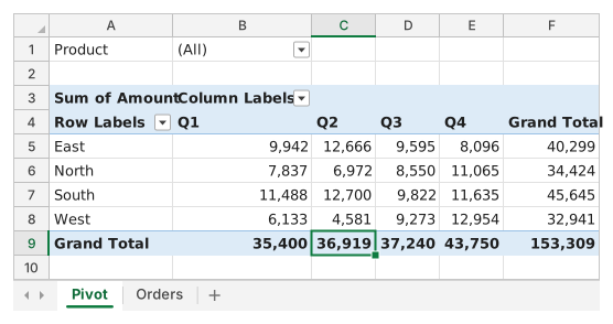
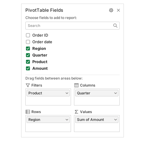
Question 1. Look at the Fields pane: which part of the report does the field in its Columns area produce?
Réponse : The Q1 to Q4 headings across the top
Quarter sits in the Columns area, and a field in Columns turns its items into the headings across the top of the report. Region in Rows gives the labels down the side, Amount in Values the numbers, and Product in Filters the (All) box above.
Question 2. What does the number in C9 of the Pivot sheet, where the Grand Total row meets the Q2 column, show?
Réponse : The Q2 amount of all four regions added together
The Grand Total row adds each column down: C9 = 12,666 + 6,972 + 12,700 + 4,581 = 36,919. The whole year of every region is the bottom-right cell F9, and a number of orders would need Count instead of Sum.
Question 3. Which region brought in the largest amount over the whole year?
Réponse : South
Read the Grand Total column (F5:F8): South has the largest year, 45,645. West owns the biggest single number in the report (12,954 in Q4) but its year adds up to only 32,941.
Question 4. You want to see the individual orders behind the East / Q3 number. What is the quickest way in Excel?
Réponse : Double-click that value cell
Double-clicking a value cell (or right-click → Show Details) puts the orders behind that number on a new worksheet. Refresh only re-reads the source data, Order ID in Values would count the orders, and PivotTable cells hold no formula to open.
Erreurs fréquentes
Typing the criteria into the formula, =SUMIFS(F2:F211,C2:C211,"East",D2:D211,"Q3"): the value matches today, but the checker switches I2 and I3 and the hard-coded formula does not follow.
Comment nous corrigeons
Toute formule qui produit le bon résultat est acceptée, sauf si la tâche nomme une fonction : une autre fonction rapporte alors la moitié des points. Nous comparons les valeurs avec une petite tolérance et ignorons la casse et les espaces dans le texte. Un nombre correct saisi à la main au lieu d’une formule rapporte la moitié des points. Les tâches sur plusieurs cellules rapportent tous les points avec 100 % de cellules justes, la moitié à partir de 50 %. Lorsque c’est pertinent, nous modifions aussi une cellule d’entrée sur une copie de votre feuille et vérifions que votre formule suit.
Réponses calculées selon les règles d’Excel 365 et vérifiées dans notre correcteur le 20 novembre 2026. Auteur : GridBelt team.