Vai al contenuto
GridBelt
  • Test Excel
  • Esercizi
  • Programmi
  • Prezzi
Accedi
Inizia il test gratuito
  • Test Excel
  • Esercizi
  • Programmi
  • Prezzi
AccediCrea un account
Inizia il test gratuito
GridBelt

Esercitati con Excel nel tuo browser.

Test Excel

  • Livello 1: Principiante
  • Livello 2: Intermedio
  • Livello 3: Esperto
  • Test Excel in 7 giorni
  • Classifica
  • Test Excel per il colloquio
  • Valutazione Excel di Indeed

Esercizi

  • Tutti gli esercizi
  • Programmi
  • Per principianti

Guide

  • Formule Excel
  • Scorciatoie Excel

Azienda

  • Chi siamo
  • Prezzi
  • Come valutiamo

© GridBelt. Tutti i diritti riservati.

  • Informativa sulla privacy
  • Termini di utilizzo
  • Politica di rimborso

Excel è un marchio di Microsoft Corporation. Indeed, TestGorilla, SHL e gli altri marchi appartengono ai rispettivi proprietari. GridBelt è un sito di esercitazione indipendente e non è affiliato a Microsoft, TestGorilla, SHL o Indeed, né approvato o sponsorizzato da queste società.

  1. Esercizi
  2. /
  3. Charts

Excel combo chart practice: revenue and margin % in one chart

  • Esperto
  • ~9 min
  • Charts

Testo dell’esercizio in inglese

An outdoor-gear shop reviews its 2026 months: revenue, cost of sales and gross profit are in A1:D13. The shop was closed for a refit in February, so that month has no sales at all. The owner wants revenue and gross margin in one chart. The first attempt (chart A) and the second (chart B) are shown below; both plot the margin column E that you are about to fill.

Two charts titled "Revenue and gross margin, 2026", each with revenue as blue columns and gross margin as an orange line with markers, January to December. Revenue: Jan $41,820, Feb $0, Mar $58,430, Apr $66,910, May $74,250, Jun $88,640, Jul $94,370, Aug $91,280, Sep $70,560, Oct $63,190, Nov $72,840, Dec $89,710. Gross margin: Jan 44.1%, Feb #N/A, Mar 35.2%, Apr 33.8%, May 36.7%, Jun 32.9%, Jul 35.8%, Aug 34.1%, Sep 39.6%, Oct 41.2%, Nov 37.4%, Dec 31.8%. In the upper chart, A, both series share one dollar axis on the left from $0 to $100,000, and the margin line runs flat along the bottom. In the lower chart, B, the dollar axis on the left is unchanged and an axis on the right runs from 0% to 50%; the margin line now rises and falls across the tops of the columns. In both charts Feb has no column and no margin point: the line breaks after Jan and starts again at Mar.

Cosa devi fare

  1. 1Gross margin is gross profit divided by revenue. Click E2 and divide D2 by B2.
  2. 2February has no revenue, so a plain division shows #DIV/0! there. Wrap it in IFERROR and give NA() as the value to show instead: the cell then shows #N/A, the value a chart leaves out.
  3. 3Fill E2 down to E13 (double-click the fill handle, or Ctrl+D / ⌘D on the selected range), then format E2:E13 as a percentage with one decimal place: Ctrl+Shift+% (Control+Shift+% on a Mac), then Increase Decimal once (in this grid: the toolbar's Increase decimal places button, under ⋮ when the toolbar is narrow; in Excel, Format Cells with Ctrl+1 / ⌘1 → Percentage → 1 decimal place works too). February stays #N/A.
  4. 4Then answer the questions about the two charts. They are pictures: this practice grid has no chart command.

Celle di risposta

Domande

Scegli qui le tue risposte: il pulsante Verifica le valuta insieme alle celle di risposta.

  1. Domanda 1In chart A, revenue and gross margin share one vertical axis. Why does the margin line lie flat along the bottom?

    Scegli una risposta.

  2. Domanda 2Chart B shows the same two series after one change. Which change was it?

    Scegli una risposta.

  3. Domanda 3In chart B the margin line has no point for February, because that margin cell holds #N/A. What would the chart show if the formula returned empty text ("") for February instead?

    Scegli una risposta.

  4. Domanda 4Which statements about chart B are true? Select all that apply.

    Seleziona tutte le risposte corrette.

Correzione

Rispondi alle domande, scrivi la formula nella griglia, premi Enter, poi Verifica. Valutiamo le tue risposte, il valore in ogni cella di risposta e la formula che lo produce.

Attività

  1. Non verificatoIn E2:E13, compute each month's gross margin, gross profit ÷ revenue, with one formula filled down; a month without revenue must return #N/A: wrap the division in IFERROR(…, NA()) (or test the revenue with IF).
  2. Non verificatoFormat E2:E13 as a percentage with one decimal place (0.0%, for example 35.2%).
  3. Non verificatoDomanda 1: In chart A, revenue and gross margin share one vertical axis. Why does the margin line lie flat along the bottom?
  4. Non verificatoDomanda 2: Chart B shows the same two series after one change. Which change was it?
  5. Non verificatoDomanda 3: In chart B the margin line has no point for February, because that margin cell holds #N/A. What would the chart show if the formula returned empty text ("") for February instead?
  6. Non verificatoDomanda 4: Which statements about chart B are true? Select all that apply.

Consigliato il computer per le attività sul foglio di calcolo. Il foglio scorre all’interno di questo riquadro.

StartInsertFormulasDataView
A1fxPreparazione della cartella di lavoro…
A
B
C
D
E
F
G
H
I
J
1
2
3
4
5
6
7
8
9
10
11
12
13
14
15
16
17
18
19
20
21
22
Sheet1

Rispondi alle domande, compila le celle, poi verifica.

Informazioni sull’esercizio

Un set di dati di 12 righe su un foglio, una cella di risposta, circa 9 minuti. Correzione nel tuo browser: il valore e la formula che lo produce, con indicazioni su cosa sistemare. L’esercizio include anche 4 domande a risposta multipla, valutate con lo stesso pulsante Verifica.

Come risolverlo

  • E2=IFERROR(D2/B2,NA())

=IFERROR(D2/B2,NA()) divides gross profit by revenue and, for February's 0 ÷ 0, returns #N/A instead of #DIV/0!; formatted as 0.0% the margins read 44.1%, 35.2% and so on. In chart A the margins (all below 0.5) share a dollar axis built for tens of thousands, so the line looks flat; chart B moves the margin to a secondary axis with its own scale from 0% to 50%. #N/A keeps February out of the line, whereas "" would be plotted as 0%. In chart B you read the margin on the right-hand axis, the crossings of line and columns mean nothing, and the best margin (January) is not the best gross profit (July).

For an existing chart, two routes in Excel 365: right-click the margin line → Format Data Series → Series Options → Secondary Axis (Windows and Mac); or select the chart → Chart Design → Change Chart Type → Combo, set Gross margin to Line and tick its Secondary Axis box (Windows). Insert → Insert Combo Chart → Clustered Column – Line on Secondary Axis builds such a chart from scratch: select A1:B13, add E1:E13 with Ctrl (⌘ on a Mac), and the margin, the second series, becomes the line. Excel 2016–2019 for Windows work the same way; the tab is called Design, under Chart Tools. Use a secondary axis for a second unit, percent next to dollars; two dollar series belong on one axis, or readers compare heights measured against different scales. Add axis titles (Chart Design → Add Chart Element → Axis Titles) so nobody reads the margin against dollars. Charts plot "" as zero, so chart data should return NA(). #N/A never becomes a point. With Select Data → Hidden and Empty Cells → Show #N/A as an empty cell ticked (new charts in Excel 365 have it on) and empty cells shown as Gaps, the line breaks at February, as in chart B; with that box cleared, it runs straight from January to March. For a table people read, a text such as n/a is friendlier (see the IFERROR margin exercise). IFERROR also hides other errors, such as a text value in a revenue cell; =IF(B2=0,NA(),D2/B2) guards only the zero.

Altri metodi validi

  • =IF(B2=0,NA(),D2/B2) — guards only the zero revenue and lets any other error show
  • =IFERROR((B2-C2)/B2,NA()) — the margin straight from revenue and cost of sales
  • =IF(ISERROR(D2/B2),NA(),D2/B2) — the pre-2007 pattern, same result

Risposte alle domande
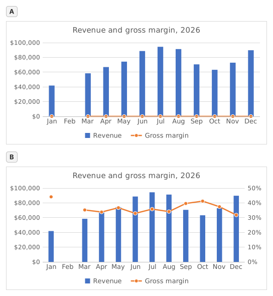
Two charts titled "Revenue and gross margin, 2026", each with revenue as blue columns and gross margin as an orange line with markers, January to December. Revenue: Jan $41,820, Feb $0, Mar $58,430, Apr $66,910, May $74,250, Jun $88,640, Jul $94,370, Aug $91,280, Sep $70,560, Oct $63,190, Nov $72,840, Dec $89,710. Gross margin: Jan 44.1%, Feb #N/A, Mar 35.2%, Apr 33.8%, May 36.7%, Jun 32.9%, Jul 35.8%, Aug 34.1%, Sep 39.6%, Oct 41.2%, Nov 37.4%, Dec 31.8%. In the upper chart, A, both series share one dollar axis on the left from $0 to $100,000, and the margin line runs flat along the bottom. In the lower chart, B, the dollar axis on the left is unchanged and an axis on the right runs from 0% to 50%; the margin line now rises and falls across the tops of the columns. In both charts Feb has no column and no margin point: the line breaks after Jan and starts again at Mar.
  1. Domanda 1. In chart A, revenue and gross margin share one vertical axis. Why does the margin line lie flat along the bottom?

    Risposta: Margins below 0.5 share an axis built for dollars

    On one axis every series uses the same scale: the axis runs to $100,000 for the revenue, so margins between 31.8% and 44.1% (0.32 to 0.44 as numbers) sit a hair above zero and every change disappears. The margin did move; it only needs its own scale.

  2. Domanda 2. Chart B shows the same two series after one change. Which change was it?

    Risposta: Gross margin series → Format Data Series → Secondary Axis

    Putting the margin on a secondary axis gives it its own scale on the right (0% to 50% here) while revenue keeps the dollar axis on the left. A Maximum of 1 would cut every revenue column off at the top, Display units only relabels the axis in thousands without changing the scale, and Switch Row/Column would turn the months into series.

  3. Domanda 3. In chart B the margin line has no point for February, because that margin cell holds #N/A. What would the chart show if the formula returned empty text ("") for February instead?

    Risposta: A point at 0% for February

    A formula that returns "" leaves text in the cell, not an empty cell, and Excel plots text in a line or column series as 0, so the line would dive to 0% in February. #N/A is never plotted as a point: chart B shows it as an empty cell, a gap (Select Data → Hidden and Empty Cells → Show #N/A as an empty cell), and with that box cleared the line would run straight from January to March, still without a February point.

  4. Domanda 4. Which statements about chart B are true? Select all that apply.

    Risposte: You read the margin on the right-hand axis e Where the line crosses a column means nothing

    The margin is plotted against the right-hand axis and the revenue against the left-hand one, so a point where the line meets a column only reflects how the two scales happen to be set. The highest margin, January's 44.1%, comes from a quiet month: July's 35.8% on far more revenue earned more gross profit ($33,780 against $18,440).

Errori comuni

Using =IFERROR(D2/B2,"") or =IFERROR(D2/B2,0): the table looks tidy, but a chart draws February at 0% and the margin line dives to the bottom; NA() keeps the month out of the chart.

Come valutiamo

È accettata qualsiasi formula che produce il risultato giusto, a meno che l’attività non indichi una funzione: in quel caso un’altra funzione vale metà dei punti. Confrontiamo i valori con una piccola tolleranza e ignoriamo maiuscole, minuscole e spazi nel testo. Un numero corretto digitato a mano invece di una formula vale metà dei punti. Le attività su più celle valgono il punteggio pieno con il 100% delle celle giuste, metà dei punti dal 50%. Dove serve, cambiamo anche una cella di input su una copia del tuo foglio e controlliamo che la formula si aggiorni.

Risposte calcolate con le regole di Excel 365 e verificate nel nostro correttore in data 20 novembre 2026. Autore: GridBelt team.

In questi programmi

  • Excel test in 7 days, Piano di livello 3Giorno 6
  • Excel for Data AnalystsGiorno 11
  • Excel for Accounting and BookkeepingGiorno 9

Esercizi correlati

  • Margin % without #DIV/0!Intermedio, ~6 min
  • Spot a misleading chart axis and measure the real differenceIntermedio, ~8 min
  • Share of total per region, formatted as %Principiante, ~5 min

Guida alla funzione

Documentazione ufficiale