Vai al contenuto
GridBelt
  • Test Excel
  • Esercizi
  • Programmi
  • Prezzi
Accedi
Inizia il test gratuito
  • Test Excel
  • Esercizi
  • Programmi
  • Prezzi
AccediCrea un account
Inizia il test gratuito
GridBelt

Esercitati con Excel nel tuo browser.

Test Excel

  • Livello 1: Principiante
  • Livello 2: Intermedio
  • Livello 3: Esperto
  • Test Excel in 7 giorni
  • Classifica
  • Test Excel per il colloquio
  • Valutazione Excel di Indeed

Esercizi

  • Tutti gli esercizi
  • Programmi
  • Per principianti

Guide

  • Formule Excel
  • Scorciatoie Excel

Azienda

  • Chi siamo
  • Prezzi
  • Come valutiamo

© GridBelt. Tutti i diritti riservati.

  • Informativa sulla privacy
  • Termini di utilizzo
  • Politica di rimborso

Excel è un marchio di Microsoft Corporation. Indeed, TestGorilla, SHL e gli altri marchi appartengono ai rispettivi proprietari. GridBelt è un sito di esercitazione indipendente e non è affiliato a Microsoft, TestGorilla, SHL o Indeed, né approvato o sponsorizzato da queste società.

  1. Esercizi
  2. /
  3. Charts

Excel chart practice: spot a misleading axis that does not start at zero

  • Intermedio
  • ~8 min
  • Charts

Testo dell’esercizio in inglese

A home-improvement chain surveys its customers every month. The regional manager's slide shows the 2026 satisfaction scores (0 to 100) of five stores as columns on a vertical axis that starts at 95, and one store looks far ahead of the rest; the manager wants to reward it. Before the meeting, measure the real difference in the sheet: the scores are in A1:B6 and the slide's axis minimum is in F2.

Two column charts titled "Customer satisfaction score, 2026" with the same five store scores, each column labelled: Harbor 98.6, Riverside 97.8, Station 95.9, Old Town 97.1, Airport 96.5. Chart A, as on the slide, has a vertical axis from 95 to 99, so each column shows only the part of the score above 95: Harbor's column towers over Station's. Chart B has a vertical axis from 0 to 100, and the five columns look almost the same height.

Cosa devi fare

  1. 1Click C2 and compare the store with the lowest score of all five: divide B2 by MIN($B$2:$B$6) and subtract 1. The $ signs keep MIN on all five stores when you fill down — F4 (Windows) or ⌘T (Mac) adds them.
  2. 2Fill C2 down to C6, then format C2:C6 as a percentage with one decimal place: Ctrl+Shift+% (Control+Shift+% on a Mac), then Increase Decimal once (in this grid: the toolbar's Increase decimal places button, under ⋮ when the toolbar is narrow; in Excel, Format Cells with Ctrl+1 / ⌘1 → Percentage → 1 decimal place works too). The lowest store shows 0.0%.
  3. 3On a chart, a column is drawn from the axis minimum up to its value, so its drawn height is the value minus the minimum. In F3, divide the drawn height of the tallest column by that of the shortest: (MAX(B2:B6) − F2) ÷ (MIN(B2:B6) − F2). Refer to F2 and do not type the minimum into the formula, so that F3 still works when the axis minimum changes.
  4. 4Then answer the questions; the charts are pictures, because this practice grid has no chart command.

Celle di risposta

Domande

Scegli qui le tue risposte: il pulsante Verifica le valuta insieme alle celle di risposta.

  1. Domanda 1On the slide (chart A), Harbor's column towers over Station's. How much higher is Harbor's score really? Use your column C.

    Scegli una risposta.

  2. Domanda 2You select the slide's vertical axis and open Format Axis (right-click the axis → Format Axis). Which change makes the columns honest?

    Scegli una risposta.

    The slide's column chart "Customer satisfaction score, 2026", narrower here, with the store names slanted; its vertical axis (95 to 99) is selected, and the Format Axis pane is open at Axis Options. Under Bounds, Minimum shows 95.0 with a Reset button next to it and Maximum shows 99.0 with an Auto button; under Units, Major shows 1.0 and Minor 0.2, both Auto.
  3. Domanda 3In which of these charts is a value axis that does not start at 0 acceptable? Select all that apply.

    Seleziona tutte le risposte corrette.

Correzione

Rispondi alle domande, scrivi la formula nella griglia, premi Enter, poi Verifica. Valutiamo le tue risposte, il valore in ogni cella di risposta e la formula che lo produce.

Attività

  1. Non verificatoIn C2:C6, compute how much higher each store's score is than the lowest of the five scores, as a share of the lowest — score ÷ lowest − 1 — with one formula filled down.
  2. Non verificatoFormat C2:C6 as a percentage with one decimal place (0.0%, for example 1.2%).
  3. Non verificatoIn F3, compute how many times taller the tallest column is drawn than the shortest on an axis that starts at the value in F2: (highest score − F2) ÷ (lowest score − F2).
  4. Non verificatoDomanda 1: On the slide (chart A), Harbor's column towers over Station's. How much higher is Harbor's score really? Use your column C.
  5. Non verificatoDomanda 2: You select the slide's vertical axis and open Format Axis (right-click the axis → Format Axis). Which change makes the columns honest?
  6. Non verificatoDomanda 3: In which of these charts is a value axis that does not start at 0 acceptable? Select all that apply.

Consigliato il computer per le attività sul foglio di calcolo. Il foglio scorre all’interno di questo riquadro.

StartInsertFormulasDataView
A1fxPreparazione della cartella di lavoro…
A
B
C
D
E
F
G
H
I
J
1
2
3
4
5
6
7
8
9
10
11
12
13
14
15
16
17
18
19
20
21
22
Sheet1

Rispondi alle domande, compila le celle, poi verifica.

Informazioni sull’esercizio

Un set di dati di 5 righe su un foglio, 2 celle di risposta, circa 8 minuti. Correzione nel tuo browser: il valore e la formula che lo produce, con indicazioni su cosa sistemare. L’esercizio include anche 3 domande a risposta multipla, valutate con lo stesso pulsante Verifica.

Come risolverlo

  • C2=B2/MIN($B$2:$B$6)-1
  • F3=(MAX(B2:B6)-F2)/(MIN(B2:B6)-F2)

Harbor's score is only 2.8% above Station's (=B2/MIN($B$2:$B$6)-1), but on an axis that starts at 95 a column only shows the part of its value above 95, so Harbor's 3.6 points against Station's 0.9 draw a column 4.0 times as tall (F3). With the axis from 0 the drawn heights are the real values and the ratio falls to 1.03. The fix is to type 0 as the axis Minimum; a non-zero axis is acceptable for lines and dots, which show values by position rather than by length.

In Excel, right-click the vertical axis → Format Axis → Axis Options → Bounds and type 0 in Minimum (the same pane on Windows and Mac, and in Excel 2016–2021). When a bound is on Auto, Excel chooses it: if the smallest value is above about five sixths of the largest, the automatic minimum is not 0, so five scores between 95.9 and 98.6 get a cut axis even if nobody set one, and Reset only returns to that automatic value. The picture shows a 300% difference where the data has 2.8%; Tufte called the ratio of the two the lie factor. When small differences matter, chart them directly: columns of each store's gap to the lowest store or to a target, a dot plot, or a line with a clearly labelled axis. Pitfall: =B2/MIN(B2:B6)-1 without $ slides the MIN range down as you fill, so the stores below Station are compared with a different "lowest" score.

Altri metodi validi

  • =B2/MIN(B$2:B$6)-1 — locking the rows is enough when you only fill down
  • =(B2-MIN($B$2:$B$6))/MIN($B$2:$B$6) — the same, written as (score − lowest) ÷ lowest
  • =(MAX(B2:B6)-$F$2)/(MIN(B2:B6)-$F$2) in F3 — the same with F2 locked

Risposte alle domande
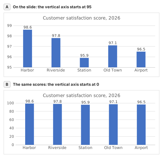
Two column charts titled "Customer satisfaction score, 2026" with the same five store scores, each column labelled: Harbor 98.6, Riverside 97.8, Station 95.9, Old Town 97.1, Airport 96.5. Chart A, as on the slide, has a vertical axis from 95 to 99, so each column shows only the part of the score above 95: Harbor's column towers over Station's. Chart B has a vertical axis from 0 to 100, and the five columns look almost the same height.
  1. Domanda 1. On the slide (chart A), Harbor's column towers over Station's. How much higher is Harbor's score really? Use your column C.

    Risposta: About 3% higher

    Harbor scores 98.6 and Station 95.9, so Harbor is 98.6 ÷ 95.9 − 1 ≈ 2.8% higher. On the slide each column only shows the part above 95: 3.6 points against 0.9, which draws Harbor's column 4.0 times as tall.

  2. Domanda 2. You select the slide's vertical axis and open Format Axis (right-click the axis → Format Axis). Which change makes the columns honest?

    Risposta: Type 0 in the Minimum box

    Columns show a value by their length from the axis, so the axis must start at 0 for the lengths to compare. Reset is not enough: when every value is above about five sixths of the largest one, as here, Excel's automatic minimum is not 0 either. Data labels print the true numbers but leave the misleading lengths.

  3. Domanda 3. In which of these charts is a value axis that does not start at 0 acceptable? Select all that apply.

    Risposte: A line chart of a share price moving between $95 and $99 e A scatter chart of house size against sale price

    Columns and bars show a value by their length, so a cut axis turns small gaps into big ones. Lines and dots show a value by its position, so their axis may zoom into the range where the values move, as long as its labels show where it starts.

Errori comuni

Filling =B2/MIN(B2:B6)-1 down without $: in the rows below Station the MIN range no longer includes Station's score, so those stores are measured against the wrong lowest store.

Come valutiamo

È accettata qualsiasi formula che produce il risultato giusto, a meno che l’attività non indichi una funzione: in quel caso un’altra funzione vale metà dei punti. Confrontiamo i valori con una piccola tolleranza e ignoriamo maiuscole, minuscole e spazi nel testo. Un numero corretto digitato a mano invece di una formula vale metà dei punti. Le attività su più celle valgono il punteggio pieno con il 100% delle celle giuste, metà dei punti dal 50%. Dove serve, cambiamo anche una cella di input su una copia del tuo foglio e controlliamo che la formula si aggiorni.

Risposte calcolate con le regole di Excel 365 e verificate nel nostro correttore in data 20 novembre 2026. Autore: GridBelt team.

Esercizi correlati

  • Read a clustered column chart of revenue by regionPrincipiante, ~6 min
  • Year-over-year % changePrincipiante, ~4 min
  • Revenue and margin % in one readable chartEsperto, ~9 min

Guida alla funzione

Documentazione ufficiale

Esercizio successivo

Series or categories? Read a chart both ways and flip its table