Pular para o conteúdo
GridBelt
  • Teste de Excel
  • Prática
  • Programas
  • Preços
Entrar
Começar o teste gratuito
  • Teste de Excel
  • Prática
  • Programas
  • Preços
EntrarCriar conta
Começar o teste gratuito
GridBelt

Pratique Excel no seu navegador.

Teste de Excel

  • Nível 1: Iniciante
  • Nível 2: Intermediário
  • Nível 3: Avançado
  • Teste de Excel em 7 dias
  • Ranking
  • Teste de Excel para entrevista
  • Avaliação de Excel da Indeed

Prática

  • Todos os exercícios
  • Programas
  • Para iniciantes

Guias

  • Fórmulas do Excel
  • Atalhos do Excel

Empresa

  • Sobre nós
  • Preços
  • Como corrigimos

© GridBelt. Todos os direitos reservados.

  • Política de Privacidade
  • Termos de Uso
  • Política de Reembolso

Excel é uma marca comercial da Microsoft Corporation. Indeed, TestGorilla, SHL e outras marcas pertencem aos seus respectivos proprietários. O GridBelt é um site de prática independente e não tem afiliação com Microsoft, TestGorilla, SHL ou Indeed, nem é endossado ou patrocinado por eles.

  1. Prática
  2. /
  3. Charts

Excel chart practice: read a clustered column chart of revenue by region

  • Iniciante
  • ~6 min
  • Charts

Enunciado em inglês

A kitchen-appliance wholesaler sells in six US regions. Before the sales kick-off, the director looks at a clustered column chart of revenue by region for 2025 and 2026, built from the table in A1:C8; the Total row adds up the regions. Read the chart to answer the questions, and put each growth rate next to the table: the chart shows dollars, not percentages.

Clustered column chart "Revenue by region ($ thousands)" with two columns per region, a blue one for 2025 and an orange one for 2026 (legend below the chart), each labelled with its value in thousands of dollars on an axis that starts at 0. Six regions from left to right, 2025 then 2026: Northeast 842 and 879; Southeast 612 and 689; Midwest 575 and 531; Southwest 403 and 446; Mountain 186 and 225; Pacific 736 and 771.

O que você precisa fazer

  1. 1The table A1:C8 holds the numbers behind the chart: one row per region with its 2025 revenue in column B and its 2026 revenue in column C, and the Total row 8.
  2. 2Click D2. Growth is the change divided by the starting year: subtract the 2025 revenue (B2) from the 2026 revenue (C2), put brackets around the difference and divide by B2.
  3. 3Press Enter and fill D2 down to D8 (double-click the fill handle or press Ctrl+D / ⌘D on the selected range), so the Total row gets the company's growth too.
  4. 4Select D2:D8 and apply a percentage format with one decimal place: Ctrl+Shift+% (Control+Shift+% on a Mac), then Increase Decimal once (in this grid: the toolbar's Increase decimal places button, under ⋮ when the toolbar is narrow; in Excel, Format Cells with Ctrl+1 / ⌘1 → Percentage → 1 decimal place works too). A fall shows as a negative percentage.
  5. 5Then answer the questions: the first three need only the chart, the last one uses your column D. The chart is a picture: this practice grid has no chart command.

Células de resposta

Questões

Escolha suas respostas aqui: o botão Verificar as corrige junto com as células de resposta.

  1. Questão 1In the chart, what do the orange columns show?

    Escolha uma resposta.

  2. Questão 2Judging by the chart, which region added the most revenue in dollars from 2025 to 2026?

    Escolha uma resposta.

  3. Questão 3Which region's revenue fell from 2025 to 2026?

    Escolha uma resposta.

  4. Questão 4Now look at your column D. Which regions grew faster in percent than the company as a whole (the Total row)? Select all that apply.

    Selecione todas as alternativas que se aplicam.

Correção

Responda às questões, digite sua fórmula na grade, pressione Enter e depois clique em Verificar. Avaliamos suas respostas, o valor de cada célula de resposta e a fórmula por trás dele.

Tarefas

  1. Não verificadoIn D2:D8, compute each row's growth from 2025 to 2026, (2026 − 2025) ÷ 2025, with one formula filled down through the Total row.
  2. Não verificadoFormat D2:D8 as a percentage with one decimal place (for example 4.4% or -7.6%).
  3. Não verificadoQuestão 1: In the chart, what do the orange columns show?
  4. Não verificadoQuestão 2: Judging by the chart, which region added the most revenue in dollars from 2025 to 2026?
  5. Não verificadoQuestão 3: Which region's revenue fell from 2025 to 2026?
  6. Não verificadoQuestão 4: Now look at your column D. Which regions grew faster in percent than the company as a whole (the Total row)? Select all that apply.

Recomendamos um computador para as tarefas de planilha. A planilha rola dentro desta caixa.

StartInsertFormulasDataView
A1fxPreparando sua pasta de trabalho…
A
B
C
D
E
F
G
H
I
J
1
2
3
4
5
6
7
8
9
10
11
12
13
14
15
16
17
18
19
20
21
22
Sheet1

Responda às questões, preencha as células e verifique.

Sobre este exercício

Um conjunto de dados de 7 linhas em uma planilha, uma célula de resposta, cerca de 6 minutos. Corrigido no seu navegador: o valor e a fórmula por trás dele, com feedback que mostra o que corrigir. O exercício também traz 4 questões de múltipla escolha, corrigidas pelo mesmo botão Verificar.

Como resolver

  • D2=(C2-B2)/B2

Growth is the change divided by the starting value: =(C2-B2)/B2 gives the first region's 2026 change as a share of 2025, and filling down to the Total row gives the company's rate to compare with; the 0.0% format shows 0.044 as 4.4%. Reading the chart: the legend says orange is 2026; the biggest dollar increase is the widest gap between a region's two columns (Southeast); the only orange column shorter than its blue partner is Midwest's; and column D shows that Southeast, Southwest and Mountain grew faster than the company.

In Excel: select A1:C7 (leave the Total row out, or its two columns dwarf every region) and choose Insert → Insert Column or Bar Chart → Clustered Column; Excel makes the two year columns the series because the range has more rows than columns. Data labels: Chart Design → Add Chart Element → Data Labels (the tab is called Design, under Chart Tools, in Excel 2016–2019); the number format code #,##0, (Format Axis or Format Data Labels → Number) shows thousands, 879,400 as 879. Pitfall 1: a chart compares heights, so it shows dollar differences; growth in percent needs the calculation, and a small region can grow fastest with the shortest columns. Pitfall 2: if the year headers were numbers instead of text, Excel could plot them as data; clearing the corner cell A1 or storing the years as text keeps them as series names (fix an existing chart with Chart Design → Select Data). Pitfall 3: =C2-B2/B2 without brackets divides first and returns a huge number instead of a percentage.

Outras formas que funcionam

  • =C2/B2-1 — the same result, shorter
  • =(C2-B2)/ABS(B2) — also right when a starting value can be negative (not the case for revenue)
  • =IFERROR((C2-B2)/B2,"") — blank instead of #DIV/0! for a region that is new this year

Respostas às questões
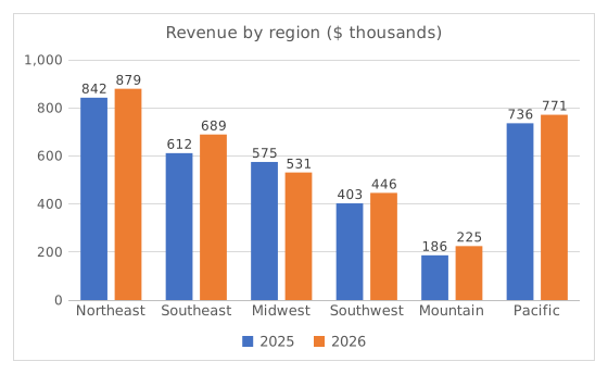
Clustered column chart "Revenue by region ($ thousands)" with two columns per region, a blue one for 2025 and an orange one for 2026 (legend below the chart), each labelled with its value in thousands of dollars on an axis that starts at 0. Six regions from left to right, 2025 then 2026: Northeast 842 and 879; Southeast 612 and 689; Midwest 575 and 531; Southwest 403 and 446; Mountain 186 and 225; Pacific 736 and 771.
  1. Questão 1. In the chart, what do the orange columns show?

    Resposta: Revenue in 2026

    The legend under the chart maps each colour to a series: blue is 2025 and orange is 2026. A clustered column chart draws one column per series in every category, side by side, so each region gets a 2025 column and a 2026 column.

  2. Questão 2. Judging by the chart, which region added the most revenue in dollars from 2025 to 2026?

    Resposta: Southeast region

    Compare the gap between each region's two columns, not the height of the orange one: Southeast goes from about 612 to 689 thousand, about $78K more, the widest gap. Northeast has the tallest columns but adds only about $37K.

  3. Questão 3. Which region's revenue fell from 2025 to 2026?

    Resposta: Midwest region

    Midwest is the only region whose orange 2026 column is shorter than its blue 2025 column (about 575 down to 531 thousand). Mountain has the shortest columns, but small is not the same as falling: its 2026 column is the taller of its pair.

  4. Questão 4. Now look at your column D. Which regions grew faster in percent than the company as a whole (the Total row)? Select all that apply.

    Respostas: Southeast region, Southwest region e Mountain region

    The company grew by 5.6%. Southeast (12.7%), Southwest (10.8%) and Mountain (20.6%) beat that. Mountain has the highest rate of all although its columns are the shortest: a percentage divides the increase by the starting value, and a small start makes a modest gain a big percentage.

Erros comuns

Typing =C2-B2/B2 without brackets: Excel divides B2 by itself first and returns the 2026 revenue minus 1 (879,399 for Northeast) instead of a growth rate. Wrap the difference in brackets: =(C2-B2)/B2.

Como corrigimos

Qualquer fórmula que produza o resultado certo é aceita, a menos que a tarefa cite uma função: nesse caso, outra função vale metade da pontuação. Comparamos os valores com uma pequena tolerância e ignoramos maiúsculas e espaços no texto. Um número certo digitado à mão em vez de uma fórmula vale metade da pontuação. Tarefas com várias células valem a pontuação integral com 100% das células certas e metade a partir de 50%. Quando faz diferença, também mudamos uma célula de entrada em uma cópia da sua planilha e verificamos se sua fórmula acompanha.

Respostas calculadas com as regras do Excel 365 e verificadas no nosso corretor em 20 de novembro de 2026. Autor: GridBelt team.

Nestes programas

  • Learn Excel From ScratchDia 2

Exercícios relacionados

  • Year-over-year % changeIniciante, ~4 min
  • Pick the right chart for each questionIniciante, ~9 min
  • Spot a misleading chart axis and measure the real differenceIntermediário, ~8 min

Referência da função

Documentação oficial

Próximo exercício

Spot a misleading chart axis and measure the real difference