Перейти к содержимому
GridBelt
  • Тест по Excel
  • Упражнения
  • Программы
  • Цены
Войти
Начать бесплатный тест
  • Тест по Excel
  • Упражнения
  • Программы
  • Цены
ВойтиСоздать аккаунт
Начать бесплатный тест
GridBelt

Тренируйте навыки Excel прямо в браузере.

Тест по Excel

  • Уровень 1: Начальный
  • Уровень 2: Средний
  • Уровень 3: Продвинутый
  • Подготовка к тесту по Excel за 7 дней
  • Таблица лидеров
  • Тест по Excel на собеседовании
  • Тест по Excel от Indeed

Упражнения

  • Все упражнения
  • Программы
  • Для начинающих

Материалы

  • Формулы Excel
  • Горячие клавиши Excel

Компания

  • О проекте
  • Цены
  • Как мы проверяем

© GridBelt. Все права защищены.

  • Политика конфиденциальности
  • Условия использования
  • Политика возврата средств

Excel — товарный знак корпорации Microsoft. Indeed, TestGorilla, SHL и другие товарные знаки принадлежат их владельцам. GridBelt — независимый сайт для практики: он не связан с Microsoft, TestGorilla, SHL или Indeed, не одобрен и не спонсируется ими.

  1. Упражнения
  2. /
  3. Charts

Excel combo chart practice: revenue and margin % in one chart

  • Продвинутый
  • ~9 мин
  • Charts

Текст упражнения на английском

An outdoor-gear shop reviews its 2026 months: revenue, cost of sales and gross profit are in A1:D13. The shop was closed for a refit in February, so that month has no sales at all. The owner wants revenue and gross margin in one chart. The first attempt (chart A) and the second (chart B) are shown below; both plot the margin column E that you are about to fill.

Two charts titled "Revenue and gross margin, 2026", each with revenue as blue columns and gross margin as an orange line with markers, January to December. Revenue: Jan $41,820, Feb $0, Mar $58,430, Apr $66,910, May $74,250, Jun $88,640, Jul $94,370, Aug $91,280, Sep $70,560, Oct $63,190, Nov $72,840, Dec $89,710. Gross margin: Jan 44.1%, Feb #N/A, Mar 35.2%, Apr 33.8%, May 36.7%, Jun 32.9%, Jul 35.8%, Aug 34.1%, Sep 39.6%, Oct 41.2%, Nov 37.4%, Dec 31.8%. In the upper chart, A, both series share one dollar axis on the left from $0 to $100,000, and the margin line runs flat along the bottom. In the lower chart, B, the dollar axis on the left is unchanged and an axis on the right runs from 0% to 50%; the margin line now rises and falls across the tops of the columns. In both charts Feb has no column and no margin point: the line breaks after Jan and starts again at Mar.

Что нужно сделать

  1. 1Gross margin is gross profit divided by revenue. Click E2 and divide D2 by B2.
  2. 2February has no revenue, so a plain division shows #DIV/0! there. Wrap it in IFERROR and give NA() as the value to show instead: the cell then shows #N/A, the value a chart leaves out.
  3. 3Fill E2 down to E13 (double-click the fill handle, or Ctrl+D / ⌘D on the selected range), then format E2:E13 as a percentage with one decimal place: Ctrl+Shift+% (Control+Shift+% on a Mac), then Increase Decimal once (in this grid: the toolbar's Increase decimal places button, under ⋮ when the toolbar is narrow; in Excel, Format Cells with Ctrl+1 / ⌘1 → Percentage → 1 decimal place works too). February stays #N/A.
  4. 4Then answer the questions about the two charts. They are pictures: this practice grid has no chart command.

Ячейки ответа

Вопросы

Ответы выбирайте здесь — кнопка «Проверить» оценит их вместе с ячейками ответа.

  1. Вопрос 1In chart A, revenue and gross margin share one vertical axis. Why does the margin line lie flat along the bottom?

    Выберите один ответ.

  2. Вопрос 2Chart B shows the same two series after one change. Which change was it?

    Выберите один ответ.

  3. Вопрос 3In chart B the margin line has no point for February, because that margin cell holds #N/A. What would the chart show if the formula returned empty text ("") for February instead?

    Выберите один ответ.

  4. Вопрос 4Which statements about chart B are true? Select all that apply.

    Выберите все подходящие варианты.

Обратная связь

Ответьте на вопросы, введите формулу в таблицу, нажмите Enter, а затем «Проверить». Мы оцениваем ваши ответы, значение в каждой ячейке ответа и формулу, которая его даёт.

Задания

  1. Не провереноIn E2:E13, compute each month's gross margin, gross profit ÷ revenue, with one formula filled down; a month without revenue must return #N/A: wrap the division in IFERROR(…, NA()) (or test the revenue with IF).
  2. Не провереноFormat E2:E13 as a percentage with one decimal place (0.0%, for example 35.2%).
  3. Не провереноВопрос 1: In chart A, revenue and gross margin share one vertical axis. Why does the margin line lie flat along the bottom?
  4. Не провереноВопрос 2: Chart B shows the same two series after one change. Which change was it?
  5. Не провереноВопрос 3: In chart B the margin line has no point for February, because that margin cell holds #N/A. What would the chart show if the formula returned empty text ("") for February instead?
  6. Не провереноВопрос 4: Which statements about chart B are true? Select all that apply.

Для заданий в таблице рекомендуем компьютер. Лист прокручивается внутри этой области.

StartInsertFormulasDataView
A1fxГотовим вашу рабочую книгу…
A
B
C
D
E
F
G
H
I
J
1
2
3
4
5
6
7
8
9
10
11
12
13
14
15
16
17
18
19
20
21
22
Sheet1

Ответьте на вопросы, заполните ячейки и проверьте.

Об этом упражнении

Набор данных (строк: 12) на одном листе, одна ячейка ответа, около 9 мин. Проверка прямо в браузере: значение и формула, которая его даёт, с обратной связью о том, что исправить. Также в упражнении есть 4 вопроса с выбором ответа — их проверяет та же кнопка «Проверить».

Как решить

  • E2=IFERROR(D2/B2,NA())

=IFERROR(D2/B2,NA()) divides gross profit by revenue and, for February's 0 ÷ 0, returns #N/A instead of #DIV/0!; formatted as 0.0% the margins read 44.1%, 35.2% and so on. In chart A the margins (all below 0.5) share a dollar axis built for tens of thousands, so the line looks flat; chart B moves the margin to a secondary axis with its own scale from 0% to 50%. #N/A keeps February out of the line, whereas "" would be plotted as 0%. In chart B you read the margin on the right-hand axis, the crossings of line and columns mean nothing, and the best margin (January) is not the best gross profit (July).

For an existing chart, two routes in Excel 365: right-click the margin line → Format Data Series → Series Options → Secondary Axis (Windows and Mac); or select the chart → Chart Design → Change Chart Type → Combo, set Gross margin to Line and tick its Secondary Axis box (Windows). Insert → Insert Combo Chart → Clustered Column – Line on Secondary Axis builds such a chart from scratch: select A1:B13, add E1:E13 with Ctrl (⌘ on a Mac), and the margin, the second series, becomes the line. Excel 2016–2019 for Windows work the same way; the tab is called Design, under Chart Tools. Use a secondary axis for a second unit, percent next to dollars; two dollar series belong on one axis, or readers compare heights measured against different scales. Add axis titles (Chart Design → Add Chart Element → Axis Titles) so nobody reads the margin against dollars. Charts plot "" as zero, so chart data should return NA(). #N/A never becomes a point. With Select Data → Hidden and Empty Cells → Show #N/A as an empty cell ticked (new charts in Excel 365 have it on) and empty cells shown as Gaps, the line breaks at February, as in chart B; with that box cleared, it runs straight from January to March. For a table people read, a text such as n/a is friendlier (see the IFERROR margin exercise). IFERROR also hides other errors, such as a text value in a revenue cell; =IF(B2=0,NA(),D2/B2) guards only the zero.

Другие рабочие способы

  • =IF(B2=0,NA(),D2/B2) — guards only the zero revenue and lets any other error show
  • =IFERROR((B2-C2)/B2,NA()) — the margin straight from revenue and cost of sales
  • =IF(ISERROR(D2/B2),NA(),D2/B2) — the pre-2007 pattern, same result

Ответы на вопросы
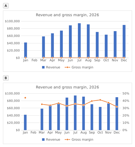
Two charts titled "Revenue and gross margin, 2026", each with revenue as blue columns and gross margin as an orange line with markers, January to December. Revenue: Jan $41,820, Feb $0, Mar $58,430, Apr $66,910, May $74,250, Jun $88,640, Jul $94,370, Aug $91,280, Sep $70,560, Oct $63,190, Nov $72,840, Dec $89,710. Gross margin: Jan 44.1%, Feb #N/A, Mar 35.2%, Apr 33.8%, May 36.7%, Jun 32.9%, Jul 35.8%, Aug 34.1%, Sep 39.6%, Oct 41.2%, Nov 37.4%, Dec 31.8%. In the upper chart, A, both series share one dollar axis on the left from $0 to $100,000, and the margin line runs flat along the bottom. In the lower chart, B, the dollar axis on the left is unchanged and an axis on the right runs from 0% to 50%; the margin line now rises and falls across the tops of the columns. In both charts Feb has no column and no margin point: the line breaks after Jan and starts again at Mar.
  1. Вопрос 1. In chart A, revenue and gross margin share one vertical axis. Why does the margin line lie flat along the bottom?

    Ответ: Margins below 0.5 share an axis built for dollars

    On one axis every series uses the same scale: the axis runs to $100,000 for the revenue, so margins between 31.8% and 44.1% (0.32 to 0.44 as numbers) sit a hair above zero and every change disappears. The margin did move; it only needs its own scale.

  2. Вопрос 2. Chart B shows the same two series after one change. Which change was it?

    Ответ: Gross margin series → Format Data Series → Secondary Axis

    Putting the margin on a secondary axis gives it its own scale on the right (0% to 50% here) while revenue keeps the dollar axis on the left. A Maximum of 1 would cut every revenue column off at the top, Display units only relabels the axis in thousands without changing the scale, and Switch Row/Column would turn the months into series.

  3. Вопрос 3. In chart B the margin line has no point for February, because that margin cell holds #N/A. What would the chart show if the formula returned empty text ("") for February instead?

    Ответ: A point at 0% for February

    A formula that returns "" leaves text in the cell, not an empty cell, and Excel plots text in a line or column series as 0, so the line would dive to 0% in February. #N/A is never plotted as a point: chart B shows it as an empty cell, a gap (Select Data → Hidden and Empty Cells → Show #N/A as an empty cell), and with that box cleared the line would run straight from January to March, still without a February point.

  4. Вопрос 4. Which statements about chart B are true? Select all that apply.

    Ответы: You read the margin on the right-hand axis и Where the line crosses a column means nothing

    The margin is plotted against the right-hand axis and the revenue against the left-hand one, so a point where the line meets a column only reflects how the two scales happen to be set. The highest margin, January's 44.1%, comes from a quiet month: July's 35.8% on far more revenue earned more gross profit ($33,780 against $18,440).

Частые ошибки

Using =IFERROR(D2/B2,"") or =IFERROR(D2/B2,0): the table looks tidy, but a chart draws February at 0% and the margin line dives to the bottom; NA() keeps the month out of the chart.

Как мы проверяем

Принимается любая формула, которая даёт верный результат, если только задание не называет функцию: тогда другая функция даёт половину балла. Мы сравниваем значения с небольшим допуском и не учитываем регистр и пробелы в тексте. Верное число, введённое вручную вместо формулы, даёт половину балла. Задания с несколькими ячейками получают полный балл, если верны 100% ячеек, и половину — если верны от 50%. Там, где это важно, мы также меняем входную ячейку в копии вашего листа и проверяем, что формула пересчитывается правильно.

Ответы рассчитаны по правилам Excel 365 и 20 ноября 2026 г. сверены в нашей системе проверки. Автор: GridBelt team.

Входит в программы

  • Excel test in 7 days, План уровня 3День 6
  • Excel for Data AnalystsДень 11
  • Excel for Accounting and BookkeepingДень 9

Похожие упражнения

  • Margin % without #DIV/0!Средний, ~6 мин
  • Spot a misleading chart axis and measure the real differenceСредний, ~8 мин
  • Share of total per region, formatted as %Начальный, ~5 мин

Справка по функции

Официальная документация