Sobre este exercício
Um conjunto de dados de 3 linhas em uma planilha, 2 células de resposta, cerca de 7 minutos. Corrigido no seu navegador: o valor e a fórmula por trás dele, com feedback que mostra o que corrigir. O exercício também traz 4 questões de múltipla escolha, corrigidas pelo mesmo botão Verificar.
Como resolver
- G1
=TRANSPOSE(A1:E4) - K2
=SUM(H2:J2)
TRANSPOSE returns the table with its rows and columns swapped: =TRANSPOSE(A1:E4) puts the quarters down column G and the models across row 1, and because it is a formula the copy follows every change in A1:E4. Each quarter then sits in one row, so its total is a plain SUM across that row. The charts: Excel made the models the series of chart A because the range has fewer models than quarters; Chart Design → Switch Row/Column turns it into chart B without touching the cells; chart B puts each model's four quarters side by side, which answers "did it grow every quarter?"; and a chart of the flipped table again gets the quarters along the axis, because Excel puts the larger number of items there.
Where it lives: select the chart, then Chart Design → Data group → Switch Row/Column (in Excel 2016–2019 the tab is called Design, under Chart Tools); Chart Design → Select Data opens the same switch together with the series and category ranges, which is where you fix a chart whose series are wrong. Excel's rule (Microsoft Support): it compares the rows and columns of the selected range and puts the larger number along the horizontal axis; with as many rows as columns, each row becomes a series. Pitfall 1: Paste Special → Transpose makes a static copy that does not follow later changes, while TRANSPOSE stays linked. Pitfall 2: an empty corner cell comes out as 0 in Excel's TRANSPOSE result; a label such as Units in A1 avoids that. Pitfall 3: in Excel 2019 and older, TRANSPOSE is a legacy array formula over a selected block (Ctrl+Shift+Enter) that you can only edit or delete as a whole; in Excel 365 it spills from one cell.
Outras formas que funcionam
- =TRANSPOSE($A$1:$E$4) in G1 — the same; the $ signs make no difference to a single formula
- =H2+I2+J2 in K2 — the same total as =SUM(H2:J2), filled down
- =SUM(B2:B4) in K2, =SUM(C2:C4) in K3 and so on — the totals straight from the original table, one formula per quarter (it cannot be filled down)
Respostas às questões
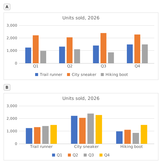
Questão 1. Chart A was inserted from A1:E4 with Excel's default settings. What did Excel make its data series?
Resposta: The three shoe models
The data series are the colours listed in the legend, one per model: Trail runner, City sneaker, Hiking boot. Excel chose them because the range has 3 model rows and 4 quarter columns: it puts the larger number of items, the 4 quarters, along the horizontal axis, so each row becomes a series.
Questão 2. Chart B shows the same cells A1:E4 as chart A. Which command turns chart A into chart B?
Resposta: Chart Design → Switch Row/Column
Switch Row/Column (Chart Design tab, Data group) swaps what the chart reads as series and as categories; the cells on the sheet stay exactly as they are. Paste Special → Transpose copies cells and leaves the chart alone, Change Chart Type changes the kind of chart, and Categories in reverse order only flips the order along the axis.
Questão 3. The sales director asks: "Did each model sell more in every quarter than in the one before?" Which chart answers that at a glance?
Resposta: Chart B
Excel draws the series of one category side by side, and neighbouring columns are the easiest to compare. In chart B each model is a category, so its four quarters stand next to each other and a steady rise shows as a staircase (Trail runner); in chart A you would have to follow one colour across four clusters. Same numbers, different comparisons made easy.
Questão 4. You insert a clustered column chart from your flipped table G1:J5 (quarters in the rows, models across) with the default settings. What does Excel put along the horizontal axis?
Resposta: The four quarters
Excel counts the rows and the columns of the range and puts the larger number of items along the horizontal axis: 4 quarters against 3 models, whichever way round the table is. So the flipped table gives the layout of chart A again; for the other layout, use Switch Row/Column on either chart.
Erros comuns
Flipping only the numbers with =TRANSPOSE(B2:E4): the labels are lost and the block lands one row and one column off, so the flipped table and the quarter totals no longer line up with the quarters.
Como corrigimos
Qualquer fórmula que produza o resultado certo é aceita, a menos que a tarefa cite uma função: nesse caso, outra função vale metade da pontuação. Comparamos os valores com uma pequena tolerância e ignoramos maiúsculas e espaços no texto. Um número certo digitado à mão em vez de uma fórmula vale metade da pontuação. Tarefas com várias células valem a pontuação integral com 100% das células certas e metade a partir de 50%. Quando faz diferença, também mudamos uma célula de entrada em uma cópia da sua planilha e verificamos se sua fórmula acompanha.
Respostas calculadas com as regras do Excel 365 e verificadas no nosso corretor em 20 de novembro de 2026. Autor: GridBelt team.