Об этом упражнении
Набор данных (строк: 3) на одном листе, 2 ячейки ответа, около 7 мин. Проверка прямо в браузере: значение и формула, которая его даёт, с обратной связью о том, что исправить. Также в упражнении есть 4 вопроса с выбором ответа — их проверяет та же кнопка «Проверить».
Как решить
- G1
=TRANSPOSE(A1:E4) - K2
=SUM(H2:J2)
TRANSPOSE returns the table with its rows and columns swapped: =TRANSPOSE(A1:E4) puts the quarters down column G and the models across row 1, and because it is a formula the copy follows every change in A1:E4. Each quarter then sits in one row, so its total is a plain SUM across that row. The charts: Excel made the models the series of chart A because the range has fewer models than quarters; Chart Design → Switch Row/Column turns it into chart B without touching the cells; chart B puts each model's four quarters side by side, which answers "did it grow every quarter?"; and a chart of the flipped table again gets the quarters along the axis, because Excel puts the larger number of items there.
Where it lives: select the chart, then Chart Design → Data group → Switch Row/Column (in Excel 2016–2019 the tab is called Design, under Chart Tools); Chart Design → Select Data opens the same switch together with the series and category ranges, which is where you fix a chart whose series are wrong. Excel's rule (Microsoft Support): it compares the rows and columns of the selected range and puts the larger number along the horizontal axis; with as many rows as columns, each row becomes a series. Pitfall 1: Paste Special → Transpose makes a static copy that does not follow later changes, while TRANSPOSE stays linked. Pitfall 2: an empty corner cell comes out as 0 in Excel's TRANSPOSE result; a label such as Units in A1 avoids that. Pitfall 3: in Excel 2019 and older, TRANSPOSE is a legacy array formula over a selected block (Ctrl+Shift+Enter) that you can only edit or delete as a whole; in Excel 365 it spills from one cell.
Другие рабочие способы
- =TRANSPOSE($A$1:$E$4) in G1 — the same; the $ signs make no difference to a single formula
- =H2+I2+J2 in K2 — the same total as =SUM(H2:J2), filled down
- =SUM(B2:B4) in K2, =SUM(C2:C4) in K3 and so on — the totals straight from the original table, one formula per quarter (it cannot be filled down)
Ответы на вопросы
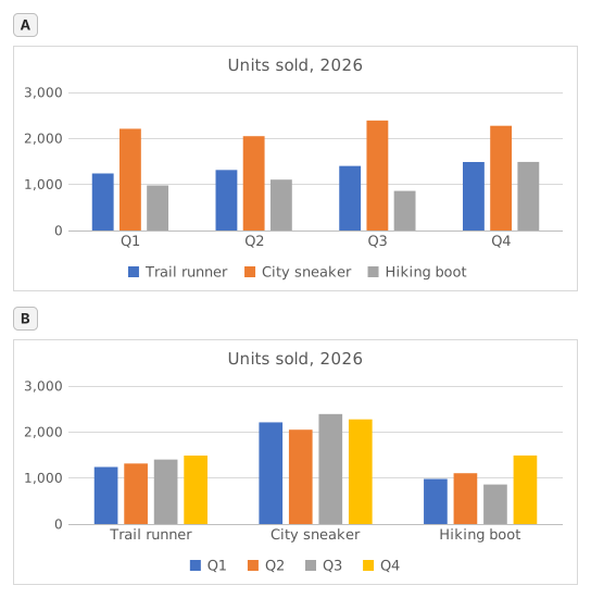
Вопрос 1. Chart A was inserted from A1:E4 with Excel's default settings. What did Excel make its data series?
Ответ: The three shoe models
The data series are the colours listed in the legend, one per model: Trail runner, City sneaker, Hiking boot. Excel chose them because the range has 3 model rows and 4 quarter columns: it puts the larger number of items, the 4 quarters, along the horizontal axis, so each row becomes a series.
Вопрос 2. Chart B shows the same cells A1:E4 as chart A. Which command turns chart A into chart B?
Ответ: Chart Design → Switch Row/Column
Switch Row/Column (Chart Design tab, Data group) swaps what the chart reads as series and as categories; the cells on the sheet stay exactly as they are. Paste Special → Transpose copies cells and leaves the chart alone, Change Chart Type changes the kind of chart, and Categories in reverse order only flips the order along the axis.
Вопрос 3. The sales director asks: "Did each model sell more in every quarter than in the one before?" Which chart answers that at a glance?
Ответ: Chart B
Excel draws the series of one category side by side, and neighbouring columns are the easiest to compare. In chart B each model is a category, so its four quarters stand next to each other and a steady rise shows as a staircase (Trail runner); in chart A you would have to follow one colour across four clusters. Same numbers, different comparisons made easy.
Вопрос 4. You insert a clustered column chart from your flipped table G1:J5 (quarters in the rows, models across) with the default settings. What does Excel put along the horizontal axis?
Ответ: The four quarters
Excel counts the rows and the columns of the range and puts the larger number of items along the horizontal axis: 4 quarters against 3 models, whichever way round the table is. So the flipped table gives the layout of chart A again; for the other layout, use Switch Row/Column on either chart.
Частые ошибки
Flipping only the numbers with =TRANSPOSE(B2:E4): the labels are lost and the block lands one row and one column off, so the flipped table and the quarter totals no longer line up with the quarters.
Как мы проверяем
Принимается любая формула, которая даёт верный результат, если только задание не называет функцию: тогда другая функция даёт половину балла. Мы сравниваем значения с небольшим допуском и не учитываем регистр и пробелы в тексте. Верное число, введённое вручную вместо формулы, даёт половину балла. Задания с несколькими ячейками получают полный балл, если верны 100% ячеек, и половину — если верны от 50%. Там, где это важно, мы также меняем входную ячейку в копии вашего листа и проверяем, что формула пересчитывается правильно.
Ответы рассчитаны по правилам Excel 365 и 20 ноября 2026 г. сверены в нашей системе проверки. Автор: GridBelt team.